Scott got a hoya earlier this year, and it is about time to transplant it into a larger pot. He wants to be able to hang it in the window to get plenty of light — so I’m making a basket to hold the plant.
The main part of the planter is 16x 18 feet strands that will be folded in half an arranged as four sets of four strands. Additionally, I need a 6.5 foot strand to wrap the hanging loop and another three foot section for gathering at the base of the loop. Wow, it takes a lot of cord to make a plant hanger.
Hanging loop followed by four groups knotted as: 7″ of spiral knot, 4.5″ straight then single knot, and
10″ of square knot. Then the groups will be changed to form a diamond shaped net that will hold our planter.
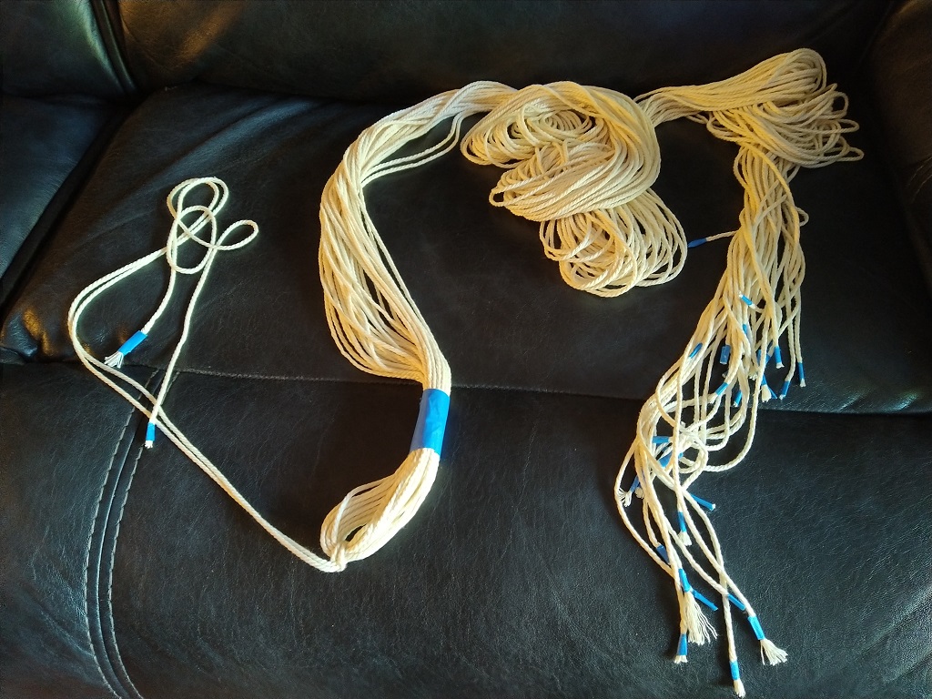
I got all of the cords cut, taped off the ends so they don’t fray, and am starting to make the hanging loop.
Since this is such a huge pile of strings, I grouped the strings that will be knotted together. Once they were grouped, I coiled each group up and used a bread time to hold the coil. I’ve still got a big pile of strings, but only the four I am actively working on are eight feet of hanging strands.
We had a Postgres server go into read-only mode — which provided a stressful opportunity to learn more nuances of Postgres internals. It appears this “read only mode” something Postgres does to save it from itself. Transaction IDs are assigned to each row in the database — the ID values are used to determine what transactions can see. For each transaction, Postgres increments the last transaction ID and assigns the incremented value to the current transaction. When a row is written, the transaction ID is stored in the row and used to determine whether a row is visible to a transaction.
Inserting a row will assign the last transaction ID to the xmin column. A transaction can see all rows where xmin is less than its transaction ID. Updating a row actually creates a new row — the old row then has an xmax value and the new row has the same number as its xmin — transactions with IDs newer than the xmax value will not see the row. Similarly, deleting a row updates the row’s xmax value — older transactions will still be able to see the row, but newer ones will not.
You can even view the xmax and xmin values by specifically asking for them in a select statement: select *, xmin, xmax from TableName;
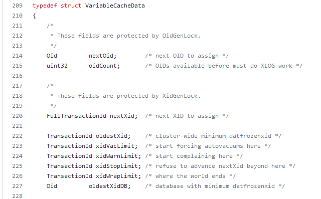
The transaction ID is stored in a 32-bit number — making the possible values 0 through 4,294,967,295. Which can become a problem for a heavily I/O or long-running database (i.e. even if I only get a couple of records an hour, that adds up over years of service) because … what happens when we get to 4,294,967,295 and need to write another record? To combat this, Postgres does something that reminds me of the “doomsday” Mayan calendar — this number range isn’t aligned on a straight line where one eventually runs into a wall. The numbers are arranged in a circle, so there’s always a new cycle and numbers are issued all over again. In the Postgres source, the wrap limit is “where the world ends”! But, like the Mayan calendar … this isn’t actually the end as much as it’s a new beginning.
How do you know if transaction 5 is ‘old’ or ‘new’ if the number can be reissued? The database considers half of the IDs in the real past and half for future use. When transaction ID four billion is issued, ID number 5 is considered part of the “future”; but when the current transaction ID is one billion, ID number 5 is considered part of the “past”. Which could be problematic if one of the first records in the database has never been updated but is still perfectly legitimate. Reserving in-use transaction IDs would make the re-issuing of transaction IDs more resource intensive (not just assign ++xid to this transaction, but xid++;is xid assigned {if so, xid++ and check again until the answer is no}; assign xid to this transaction). Instead of implementing more complex logic, rows can be “frozen” — this is a special flag that basically says “I am a row from the past and ignore my transaction ID number”. In versions 9.4 and later, both committed and aborted hint bits are set to freeze a row — in earlier versions, used a special FrozenTransactionId index.
There is a minimum age for freezing a row — it generally doesn’t make sense to mark a row that’s existed for eight seconds as frozen. This is configured in the database as the vacuum_freeze_min_age. But it’s also not good to let rows sit around without being frozen for too long — the database could wrap around to the point where the transaction ID is reissued and the row would be lost (well, it’s still there but no one can see it). Since vacuuming doesn’t look through every page of the database on every cycle, there is a vacuum_freeze_table_age which defines the age of a transaction where vacuum will look through an entire table to freeze rows instead of relying on the visibility map. This combination, hopefully, balances the I/O of freezing rows with full scans that effectively freeze rows.
What I believe led to our outage — most of our data is time-series data. It is written, never modified, and eventually deleted. Auto-vacuum will skip tables that don’t need vacuuming. In our case, that’s most of the tables. The autovacuum_freeze_max_age parameter sets an ‘age’ at which vacuuming is forced. If these special vacuum processes don’t complete fully … you eventually get into a state where the server stops accepting writes in order to avoid potential data loss.
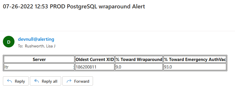
So monitoring for transaction IDs approaching the wraparound and emergency vacuum values is important. I set up a task that alerts us when we approach wraparound (fortunately, we’ve not gotten there again) as well as when we approach the emergency auto-vacuum threshold — a state which we reach a few times a week.
Using the following query, we monitor how close each of our databases is to both the auto-vacuum threshold and the ‘end of the world’ wrap-around point.
WITH max_age AS ( SELECT 2000000000 as max_old_xid
                        , setting AS autovacuum_freeze_max_age FROM pg_catalog.pg_settings
                        WHERE name = 'autovacuum_freeze_max_age' )
         , per_database_stats AS ( SELECT datname , m.max_old_xid::int
                        , m.autovacuum_freeze_max_age::int
                        , age(d.datfrozenxid) AS oldest_current_xid
                        FROM pg_catalog.pg_database d
                        JOIN max_age m ON (true) WHERE d.datallowconn )

SELECT max(oldest_current_xid) AS oldest_current_xid
      , max(ROUND(100*(oldest_current_xid/max_old_xid::float))) AS percent_towards_wraparound
      , max(ROUND(100*(oldest_current_xid/autovacuum_freeze_max_age::float))) AS percent_towards_emergency_autovac FROM per_database_stats
If we are approaching either point, e-mail alerts are sent.
When a database approaches the emergency auto-vacuum threshold, we freeze data manually — vacuumdb --all --freeze --jobs=1 --echo --verbose --analyze (or –jobs=3 if I want the process to hurry up and get done).
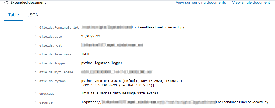
I’ve been working on forking log data into two different indices based on an element contained within the record — if the filename being sent includes the string “BASELINE”, then the data goes into the baseline index, otherwise it goes into the scan index. The data being ingested has the file name in “@fields.myfilename”
It took a while to figure out how to get the value from the current data — event.get(‘[@fields][myfilename]’) to get the @fields.myfilename value.
The following logstash config accepts JSON inputs, parses the underscore-delimited filename into fields, replaces the dashes with underscores as KDL doesn’t handle dashes and wildcards in searches, and adds a flag to any record that should be a baseline. In the output section, that flag is then used to publish data to the appropriate index based on the baseline flag value.
We checked on the bees around noon today. We’ve seen a lot of activity at the hive, and they seem to love the field of clover in our yard — so we were curious to see how much the colony had built up. It wasn’t as full as we were hoping (we would have loved to add a super!). There were more bees in the upper deep than last time, but the hive box wasn’t super full. Maybe five frames with brood, several frames with honey, and a few frames that they’d started drawing out. We moved the frames around — the brood frames were all clustered together, so we moved (2?) frames up to the top deep and interspersed empty and half-empty frames with the full ones. Hopefully having empty frames in the middle will encourage them to build out the frames.
There’s often a difference between hypothetical (e.g. the physics formula answer) and real results — sometimes this is because sciences will ignore “negligible” factors that can be, well, more than negligible, sometimes this is because the “real world” isn’t perfect. In transmission media, this difference is a measurable “loss” — hypothetically, we know we could send X data in Y delta-time, but we only sent X’. Loss also happens because stuff breaks — metal corrodes, critters nest in fiber junction boxes, dirt builds up on a dish. And it’s not easy, when looking at loss data at a single point in time, to identify what’s normal loss and what’s a problem.
We’re starting a project to record a baseline of loss for all sorts of things — this will allow individuals to check the current loss data against that which engineers say “this is as good as it’s gonna get”. If the current value is close … there’s not a problem. If there’s a big difference … someone needs to go fix something.
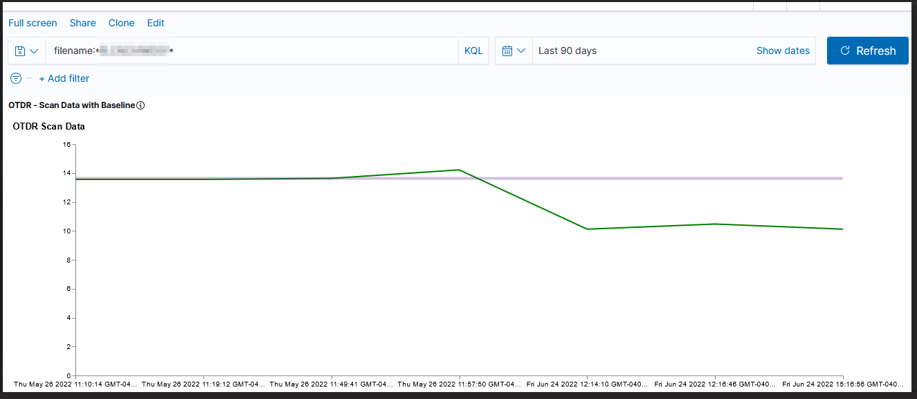
Unfortunately, creating a graph in Kibana that shows the baseline was … not trivial. There is a rule mark that allows you to draw a straight line between two points. You cannot just say “draw a line at y from 0 to some large value that’s going to be off the graph. The line doesn’t render (say, 0 => today or the year 2525). You cannot just get the max value of the axis.
I finally stumbled across a series of data contortions that make the baseline graphable.
The data sets I have available have a datetime object (when we measured this loss) and a loss value. For scans, there may be lots of scans for a single device. For baselines, there will only be one record.
The joinaggregate transformation method — which appends the value to each element of the data set — was essential because I needed to know the largest datetime value that would appear in the chart.
The lookup transformation method — which can access elements from other data sets — allowed me to get that maximum timestamp value into the baseline data set. Except … lookup needs an exact match in the search field. Luckily, it does return a random (I presume either first or last … but it didn’t matter in this case because all records have the same max date value) record when multiple matches are found.
Voila — a chart with a horizontal line at the baseline loss value. Yes, I randomly copied a record to use as the baseline and selected the wrong one (why some scans are below the “good as it’s ever going to get” baseline value!). But … once we have live data coming into the system, we’ll have reasonable looking graphs.
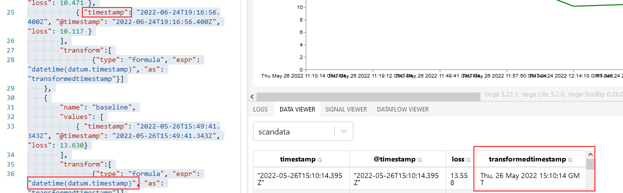
We have data created by an external source (i.e. I cannot just change the names used so it works) — the datetime field is named @timestamp and I had an awful time figuring out out how to address that element within a transformation expression.
Just to make sure I wasn’t doing something silly, I created a copy of the data element named without the at symbol. Voila – transformedtimestamp is populated with a datetime element.
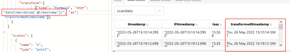
I finally figured it out – it appears that I have encountered a JavaScript limitation. Instead of using the dot-notation to access the element, the array subscript method works – not datum.@timestamp in any iteration or with any combination of escapes.
Preheat oven to 325F. Whisk all ingredients together and pour into individual ramekins. Fill a baking pan with some water, place ramekins into pan. Bake until the custard sets — about 30 minutes.
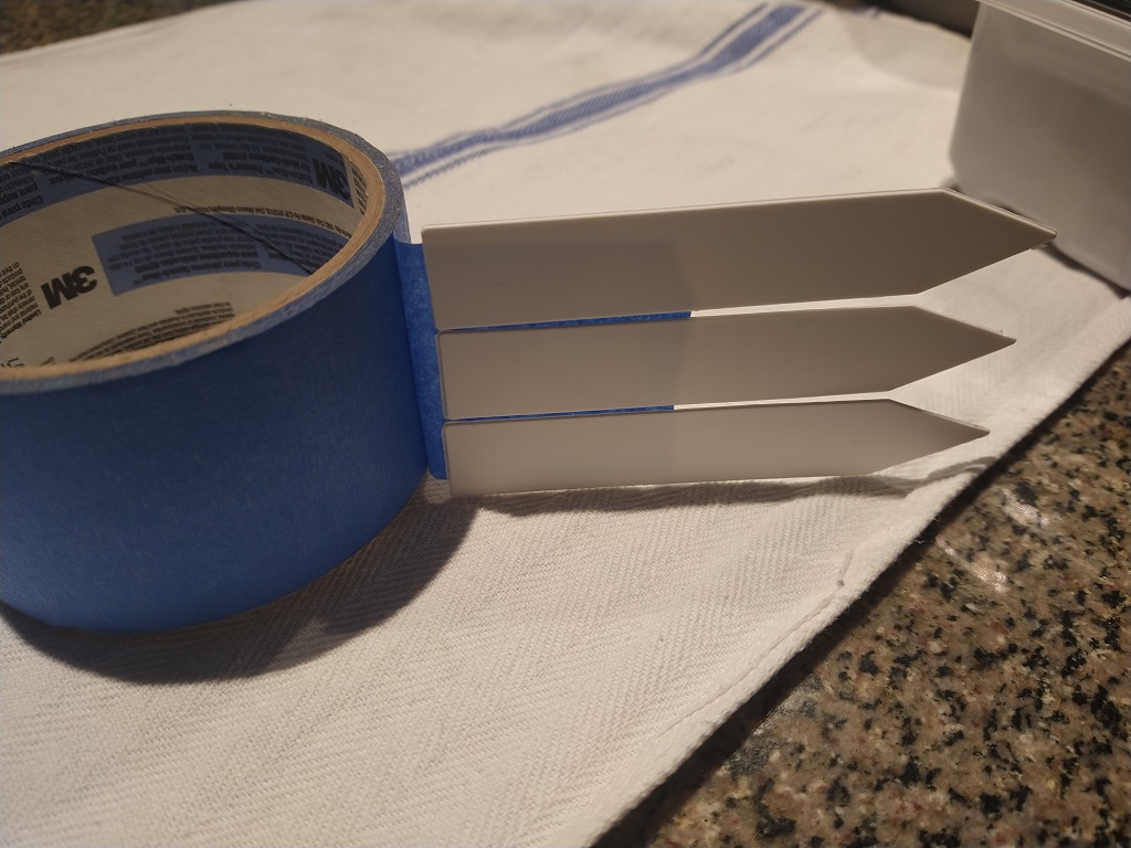
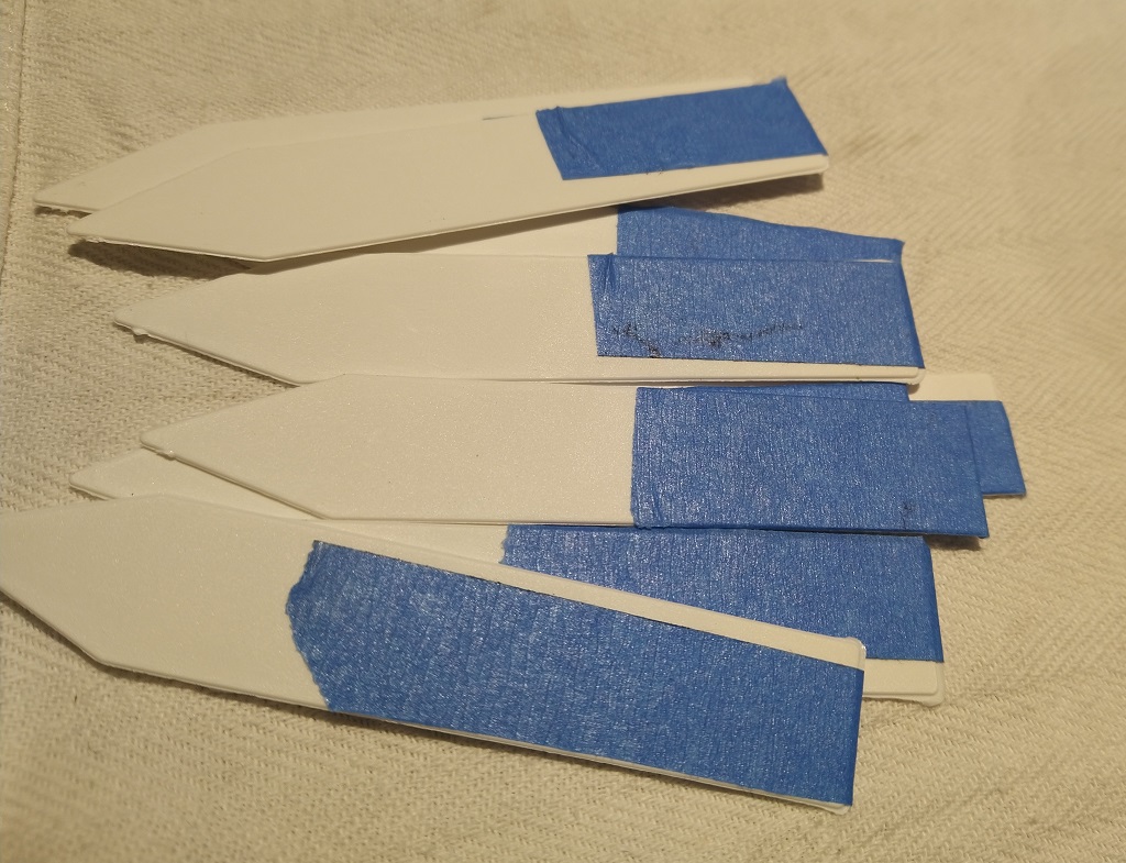
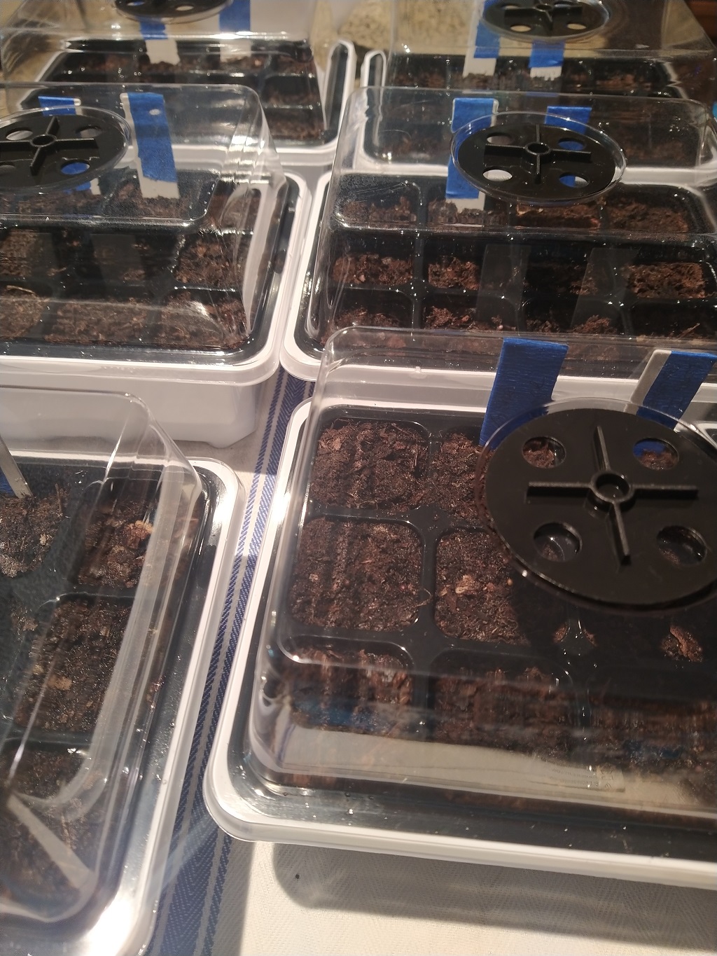
I got the seeds started for our fall harvested vegetables. We bought these little seed starting trays on Amazon — a tray, a 12-cell insert, and a humidity dome with an adjustable vent. The kit came with plant markers … but it seemed silly to write something permanent on the marker. So I turned them into reusable markers by adding some of the blue tape you use for painting a room (because that’s what we’ve got & pen works OK on it). First I put three of the markers in a line on the tape.
Making plant labels reusable
A couple of quick slices with an Exacto knife, and I can change the label as needed.
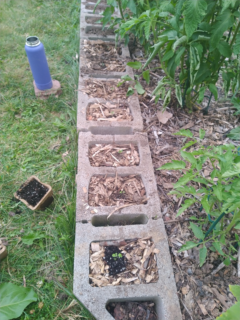
When we decided to use some old cinder blocks to build raised beds, the idea was to fill all of the blocks with dirt and use the spaces as bonus planting spaces for small plants like flowers and herbs. Functional and aesthetically pleasing. I never got far in that project — filled some blocks with dirt and lots of weeds. But no ring of herbs around the bed.
This year, I’m doing it! It’s a time consuming process to clear out the existing plant growth. I’m adding about two inches of rocks (we’ve got a lot of rock-covered beds that we want to de-rock), and filling up with soil. Anya started a bunch of herb plants, so she has been transplanting her seedlings into the blocks and adding some wood mulch (I expect these small blocks will warm up and dry out rather quickly otherwise).