I don’t remember when we saw the first fireflies — walking back to the house after dark, there was one lonely little flash out in the field. But, over the past week or so, that one flash has been joined by dozens of others.

I don’t remember when we saw the first fireflies — walking back to the house after dark, there was one lonely little flash out in the field. But, over the past week or so, that one flash has been joined by dozens of others.
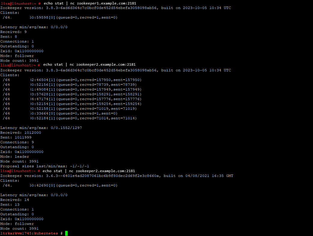
Provided you have stat enabled (something like 4lw.commands.whitelist=stat, in ./config/zookeeper.properties), you can use nc to send stat to each zookeeper and verify it is working. You can also tell which is the leader and how many clients (your current request is one!) are attached to each zookeeper node.
We got most of the north side of the garden planted — watermelon and tomatoes are still in the greenhouse (sprouting)
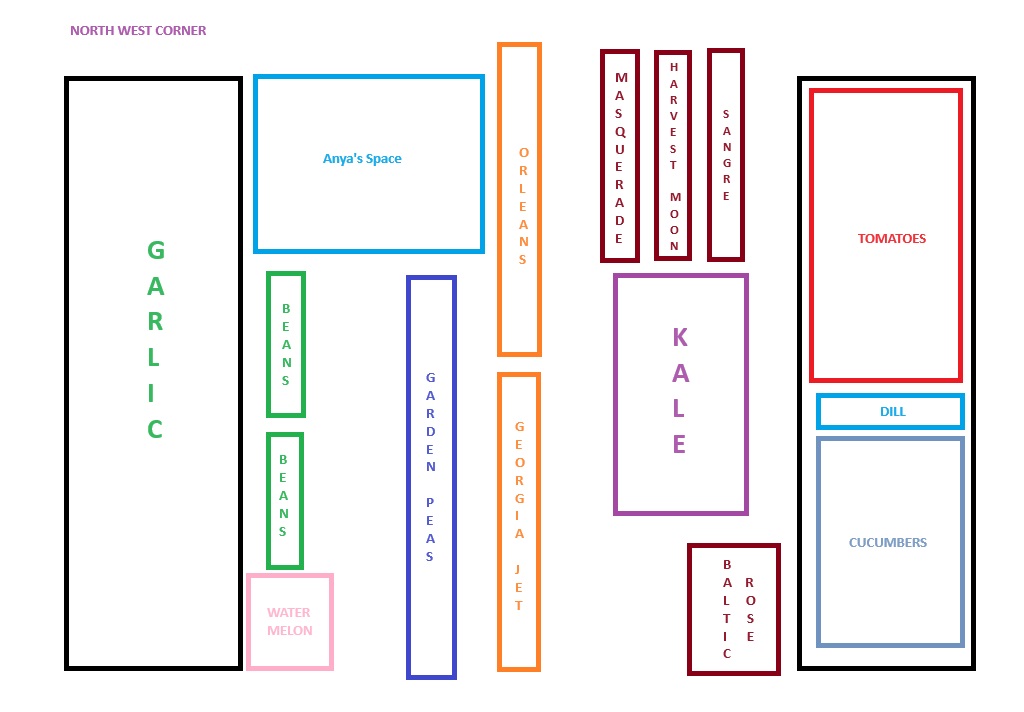
Today, we planted (from West to East) haricot vert beans, a row of peas, sweet potatoes, and regular potatoes (Masquerade, Harvest Moon, and Sangre from W to E along the north side of the kale island, and Baltic Rose along the south side of the kale)
This process presumes you have generated a signing key (/root/signing/MOK.priv and /root/signing/MOK.der) that has been registered for signing modules.
################################################################################
## Install from Repo and Sign Modules
################################################################################
yum install https://dl.fedoraproject.org/pub/epel/epel-release-latest-8.noarch.rpm
yum install kernel-devel

# Install kmod version of ZS
yum install https://zfsonlinux.org/epel/zfs-release-2-3$(rpm --eval "%{dist}").noarch.rpm
dnf config-manager --disable zfs
dnf config-manager --enable zfs-kmod
yum install zfs

# And autoload
echo zfs >/etc/modules-load.d/zfs.conf

# Use rpm -ql to list out the kernel modules that this version of ZFS uses -- 2.1.x has quite a few of them, and they each need to be signed
# Sign zfs.ko and spl.ko in current kernel
/usr/src/kernels/$(uname -r)/scripts/sign-file sha256 /root/signing/MOK.priv /root/signing/MOK.der /lib/modules/$(uname -r)/weak-updates/zfs/zfs/zfs.ko
/usr/src/kernels/$(uname -r)/scripts/sign-file sha256 /root/signing/MOK.priv /root/signing/MOK.der /lib/modules/$(uname -r)/weak-updates/zfs/spl/spl.ko
# And sign the bunch of other ko files in the n-1 kernel rev (these are symlinked from the current kernel)
/usr/src/kernels/$(uname -r)/scripts/sign-file sha256 /root/signing/MOK.priv /root/signing/MOK.der /lib/modules/4.18.0-513.18.1.el8_9.x86_64/extra/zfs/avl/zavl.ko
/usr/src/kernels/$(uname -r)/scripts/sign-file sha256 /root/signing/MOK.priv /root/signing/MOK.der /lib/modules/4.18.0-513.18.1.el8_9.x86_64/extra/zfs/icp/icp.ko
/usr/src/kernels/$(uname -r)/scripts/sign-file sha256 /root/signing/MOK.priv /root/signing/MOK.der /lib/modules/4.18.0-513.18.1.el8_9.x86_64/extra/zfs/lua/zlua.ko
/usr/src/kernels/$(uname -r)/scripts/sign-file sha256 /root/signing/MOK.priv /root/signing/MOK.der /lib/modules/4.18.0-513.18.1.el8_9.x86_64/extra/zfs/nvpair/znvpair.ko
/usr/src/kernels/$(uname -r)/scripts/sign-file sha256 /root/signing/MOK.priv /root/signing/MOK.der /lib/modules/4.18.0-513.18.1.el8_9.x86_64/extra/zfs/unicode/zunicode.ko
/usr/src/kernels/$(uname -r)/scripts/sign-file sha256 /root/signing/MOK.priv /root/signing/MOK.der /lib/modules/4.18.0-513.18.1.el8_9.x86_64/extra/zfs/common/zcommon.ko
/usr/src/kernels/$(uname -r)/scripts/sign-file sha256 /root/signing/MOK.priv /root/signing/MOK.der /lib/modules/4.18.0-513.18.1.el8_9.x86_64/extra/zfs/zstd/zzstd.ko

# Verify they are signed now
modinfo -F signer /usr/lib/modules/$(uname -r)/weak-updates/zfs/zfs/zfs.ko
modinfo -F signer /usr/lib/modules/$(uname -r)/weak-updates/zfs/spl/spl.ko

modinfo -F signer /lib/modules/4.18.0-513.18.1.el8_9.x86_64/extra/zfs/avl/zavl.ko
modinfo -F signer /lib/modules/4.18.0-513.18.1.el8_9.x86_64/extra/zfs/icp/icp.ko
modinfo -F signer /lib/modules/4.18.0-513.18.1.el8_9.x86_64/extra/zfs/lua/zlua.ko
modinfo -F signer /lib/modules/4.18.0-513.18.1.el8_9.x86_64/extra/zfs/nvpair/znvpair.ko
modinfo -F signer /lib/modules/4.18.0-513.18.1.el8_9.x86_64/extra/zfs/unicode/zunicode.ko
modinfo -F signer /lib/modules/4.18.0-513.18.1.el8_9.x86_64/extra/zfs/zcommon/zcommon.ko
modinfo -F signer /lib/modules/4.18.0-513.18.1.el8_9.x86_64/extra/zfs/zstd/zzstd.ko

# Reboot
init 6

# And we've got ZFS, so create the pool
zpool create pgpool sdc
zfs create zpool/zdata
zfs set compression=lz4 zpool/zdata

zfs get compressratio zpool/zdata
zfs set mountpoint=/zpool/zdata zpool/zdata
What happens if you only sign zfs.ko? All sorts of errors that look like there’s some sort of other problem — zfs will not load. It will tell you the required key is not available
May 22 23:42:44 sandboxserver systemd-modules-load[492]: Failed to insert 'zfs': Required key not available
Using insmod to try to manually load it will tell you there are dozens of unknown symbols:
May 22 23:23:23 sandboxserver kernel: zfs: Unknown symbol ddi_strtoll (err 0)
May 22 23:23:23 sandboxserver kernel: zfs: Unknown symbol spl_vmem_alloc (err 0)
May 22 23:23:23 sandboxserver kernel: zfs: Unknown symbol taskq_empty_ent (err 0)
May 22 23:23:23 sandboxserver kernel: zfs: Unknown symbol zone_get_hostid (err 0)
May 22 23:23:23 sandboxserver kernel: zfs: Unknown symbol tsd_set (err 0)
But the real problem is that there are unsigned modules so … there are unknown symbols. But not because something is incompatible. Just because the module providing that symbol will not load.
This process presumes you have generated a signing key (/root/signing/MOK.priv and /root/signing/MOK.der) that has been registered for signing modules.
# Install prerequisites
dnf install --skip-broken epel-release gcc make autoconf automake libtool rpm-build libtirpc-devel libblkid-devel libuuid-devel libudev-devel openssl-devel zlib-devel libaio-devel libattr-devel elfutils-libelf-devel kernel-devel-$(uname -r) python3 python3-devel python3-setuptools python3-cffi libffi-devel git ncompress libcurl-devel

dnf install --skip-broken --enablerepo=epel --enablerepo=powertools python3-packaging dkms

# Clone OpenZFS repo
git clone https://github.com/openzfs/zfs
cd zfs
# generally stay in the main branch, but if you want to use the latest then check out the staging branch
# git checkout zfs-2.2.5-staging
./autogen.sh
./configure
make
make install

# Sign the kernel modules
/usr/src/kernels/$(uname -r)/scripts/sign-file sha256 /root/signing/MOK.priv /root/signing/MOK.der /lib/modules/$(uname -r)/extra/zfs.ko
/usr/src/kernels/$(uname -r)/scripts/sign-file sha256 /root/signing/MOK.priv /root/signing/MOK.der /lib/modules/$(uname -r)/extra/spl.ko

# And verify the modules are signed
modinfo -F signer /usr/lib/modules/$(uname -r)/extra/zfs.ko
modinfo -F signer /usr/lib/modules/$(uname -r)/extra/spl.ko
The new servers being built at work use SecureBoot — something that you don’t even notice 99% of the time. But that 1% where you are doing something “strange” like trying to use OpenZFS … well, you’ve got to sign any kernel modules that you need to use. Just installing them doesn’t work — they won’t load.
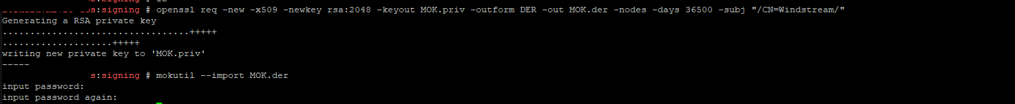
To sign a kernel module, first you need to create a signing key and use mokutil to import it into the machine owner key store.
cd /root
mkdir signing
cd signing
openssl req -new -x509 -newkey rsa:2048 -keyout MOK.priv -outform DER -out MOK.der -nodes -days 36500 -subj "/CN=MyOrg/"

mokutil --import MOK.der
When you run mokutil, you will set a password. This password will be needed to complete importing the key to the machine.
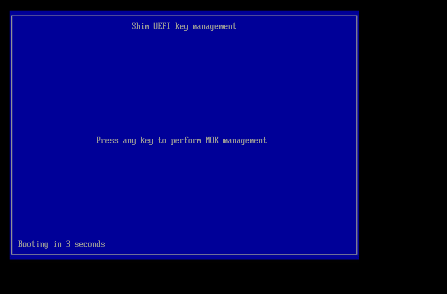
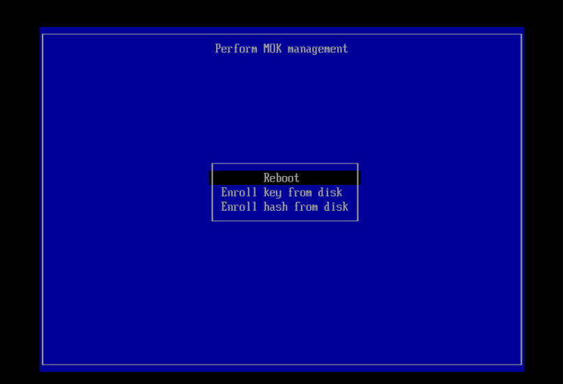
Get access to the console — out of band management, vSphere manager, stand in front of the server. Reboot, and there will be a “press any key” screen for ten seconds that begins the import process. Press any key!
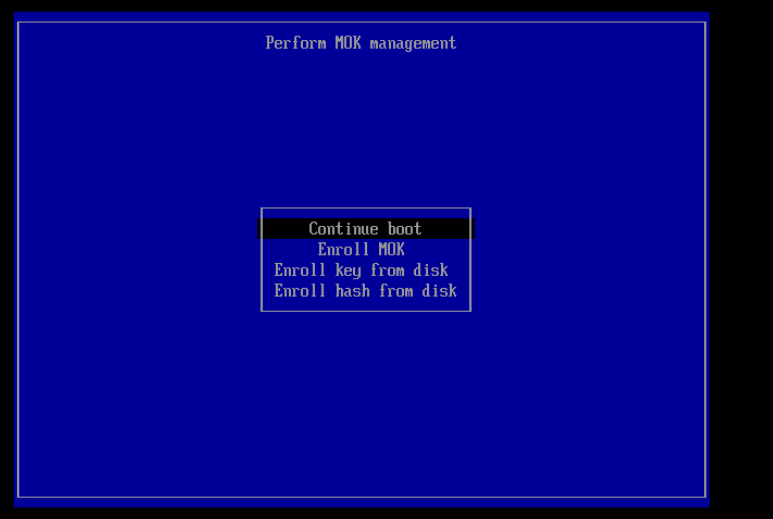
Select “Enroll MOK”
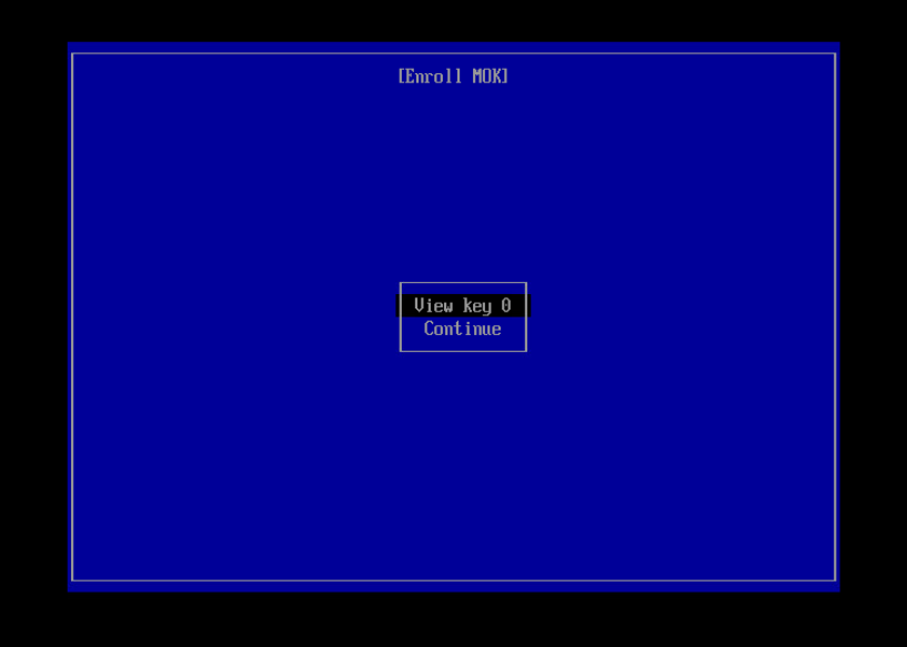
View the key and verify it is the right one, then use ‘Continue’ to import it
Enter the password used when you ran mokutil
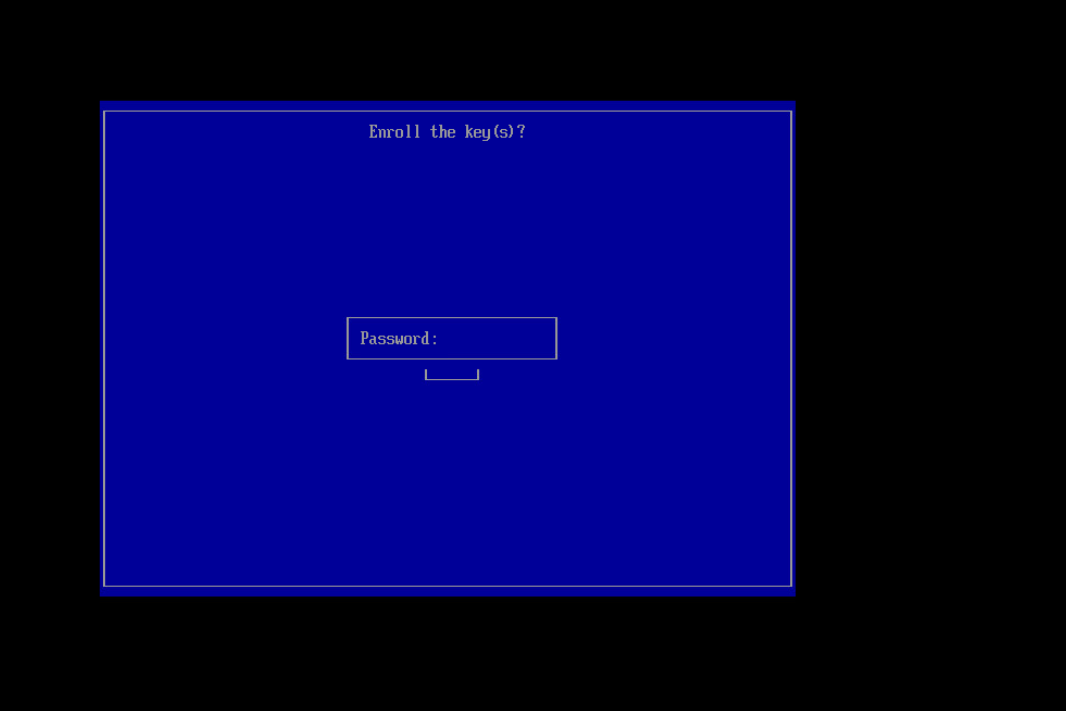
Then reboot
To verify your key has been successfully enrolled:
mokutil --list-enrolled
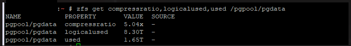
Our database storage is sizable. To reduce the financial impact of storing so much data, we opted to use a compressed file system. This allows us to maintain, for example, 8TB of data in under 2TB of space. Unfortunately, the ZFS file system we use to compress our data is no longer “built in” with newer version of RedHat.
There are alternatives. BTRFS is a long-standing option, however it’s got reliability issues (we piloted BTRFS on one of the read only replicas, and the compression ratio is nowhere near as good — the 2TB of ZFS data filled the 10TB BTRFS disk even using the better compression option. And I/O was so slow there was a continual replication backlog). RedHat introduced Virtual Disk Optimizer to replace ZFS. In theory, it’s better since it also deduplicates data (e.g. if every one of us saved the same PPT presentation to the disk, only one copy would actually be stored). That’s great for email and file shares where a lot of people are likely to store the same information. Not so useful on a database server where there’s little to de-duplicate. It does, however, compress data … so we decided to try it out.
The results, unfortunately, are not spectacular. VDO does not allow you to do much customization of the compression. It’s on or off. I’ve found some people tweaking it up in unsupported ways, but the impetus behind trying VDO was that it’s supported by RedHat. Making unsupported changes to it defeats that purpose. And the compression that we’re seeing is far less than we get in ZFS. Our existing servers run between 4.5x and 6x compression
In VDO, however, we don’t even get a 2x compression factor. 11TB of information is stored in 8TB of space! That’s 1.4x
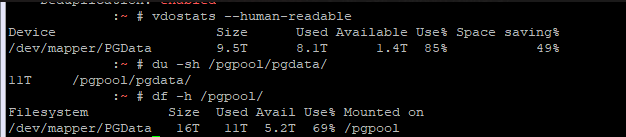
So, while we found the performance of VDO to be satisfactory and it’s really easy to use in newer RedHat releases … we’d have to increase our 20TB LUNs to 80TB to continue storing the data we store today. That seems like A Really Bad Idea(tm).
Seems like I’m going to have to sort out using OpenZFS on the new servers.
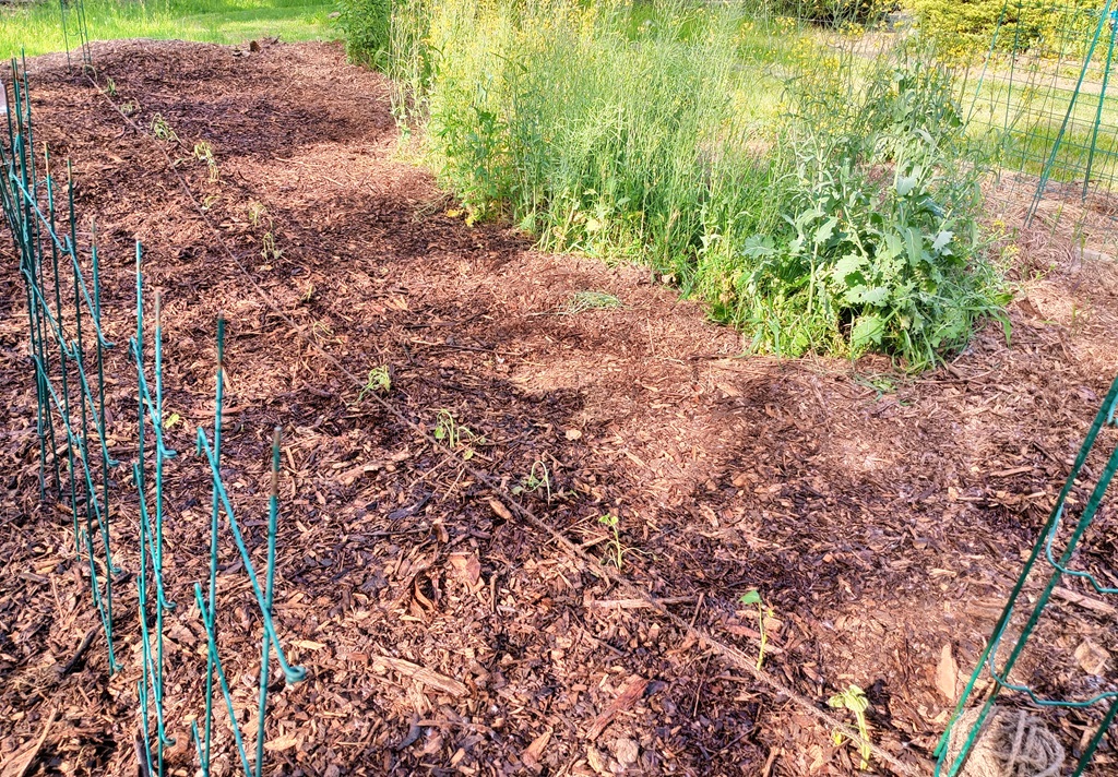
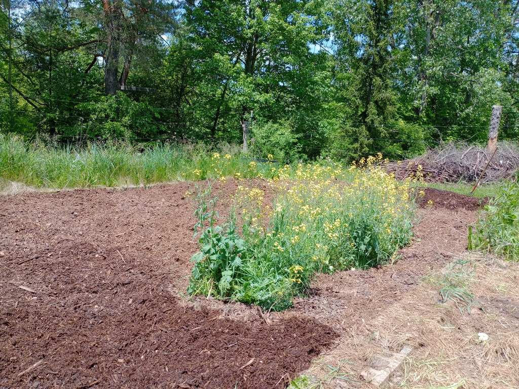
I finally got the dirt and mulch spread out in the northern side of the garden — there’s a nice island of kale in the middle, and the garlic we planted last year is growing well in the back. I’ve got potatoes and yams to plant, beans, peas, cucumbers, dill, and tomatoes. Hopefully lots and lots of tomatoes! Oh, and watermelon.
I often need to quickly see if a cert is going to expire — I’ve got nice monitoring scripts too, but something that I can run from the command line right now
echo -n Q | openssl s_client -connect $HOST:$PORT | openssl x509 -noout -dates