The default size limit for CSV reports in Kibana is 10 meg. Since that’s not enough for some of our users, I’ve been testing increases to the xpack.reporting.csv.maxSizeBytes value.
We’re still limited by the ES http.max_content_length value — which the documentation seems pretty confident shouldn’t be increased because the system can become unstable. Increasing the max Kibana report size to 100mb just yields a different error because ES doesn’t like it. 75 exhausted the JavaScript heap (?) – which I could get around by setting NODE_OPTIONS=–max_old_space_size=4096 … but that just led to the server abending whenever a report was run (in fact, I had to remove the reports I tried to run from the server to get everything back into a working state). Increasing the limit to 50 meg, though, didn’t do anything unreasonable in dev. So somewhere between 50 and 75 meg is our upper limit, and 50 seemed like a nice round number to me.
Notes on resource usage – Data is held in memory as a report is created. We’d see an increase in memory/CPU usage while the report is being generated (or, I guess more accurately, a longer time during which the memory/CPU usage is increased because if a 10 meg report takes 30 seconds to run then a 50 meg report is going to take 2.5 minutes to run … and the memory/CPU usage is pretty much the same during the “a report is running” period).
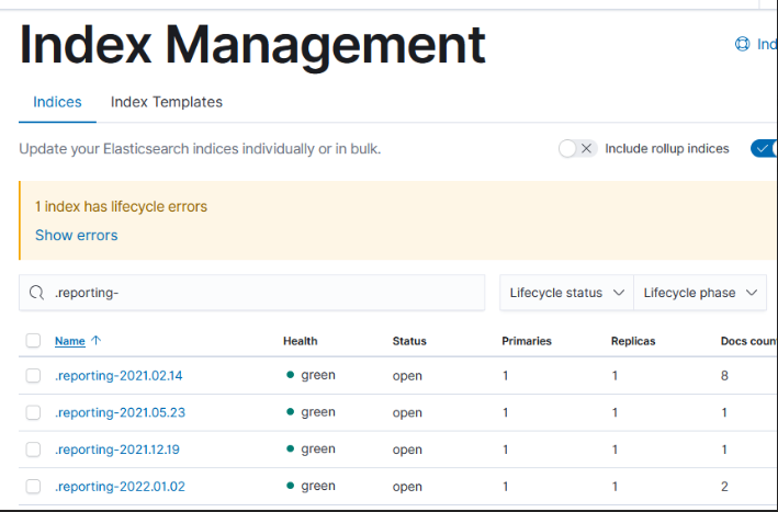
Then, though, the report is stashed in ElasticSearch for user(s) to retrieve within .reporting* indicies. And that’s where things get a little silly — architecturally, this is just another index; it ages off with a lifecycle policy if one exists. But it looks like they never created a lifecycle management policy. So you can still retrieve reports run a little over two years ago! We will certainly want to set up a policy to clean up old reports … just have to decide how long is reasonable.
Before we can use map details in Kibana visualizations, we need to add fields with the geographic information. The first few steps are something the ELK admin staff will need to do in order to map source and/or destination IPs to geographic information.
First update the relevant index template to map the location information into geo-point fields – load this JSON (but, first, make sure there aren’t existing mappings otherwise you’ll need to merge the existing JSON in with the new elements for geoip_src and geoip_dst
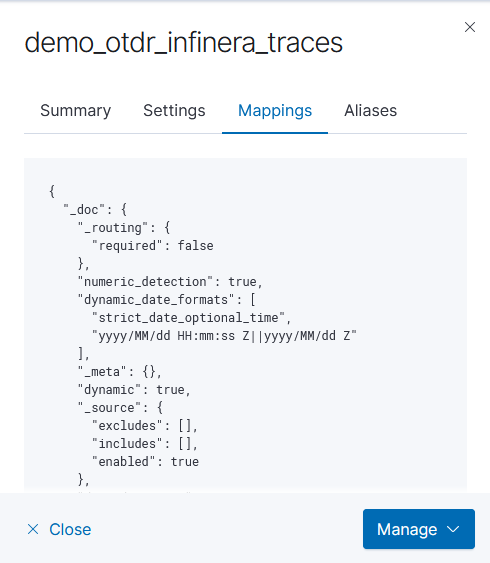
First, click on the index template name to view the settings. Click to the ‘mappings’ tab and copy what is in there
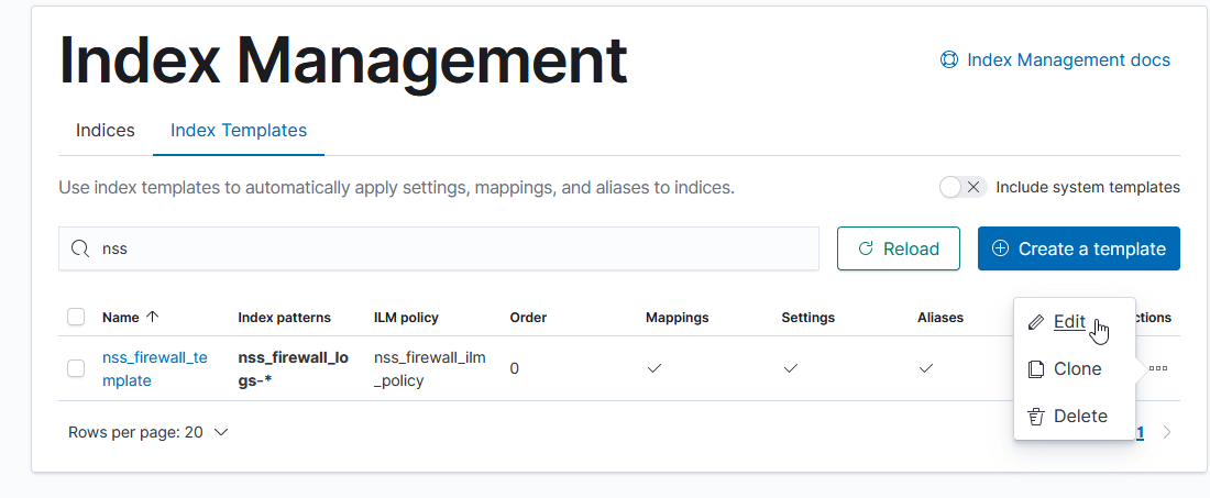
Munge in the two ‘properties’ in the above JSON. Edit the index template
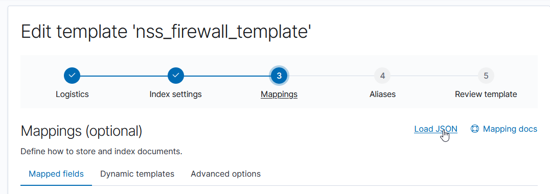
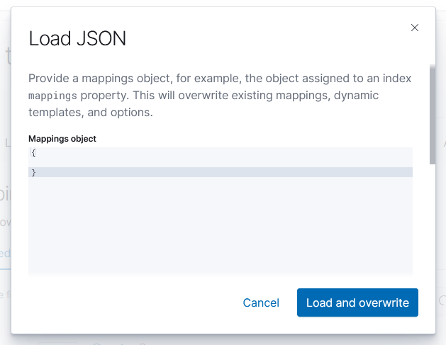
Click to the “Mappings” section and use “Load JSON” to import the new mapping configuration
Paste in your JSON & click to “Load & Overwrite”
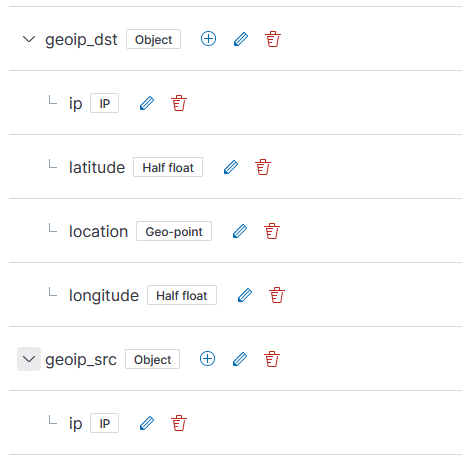
Voila – you will have geo-point items in the template.
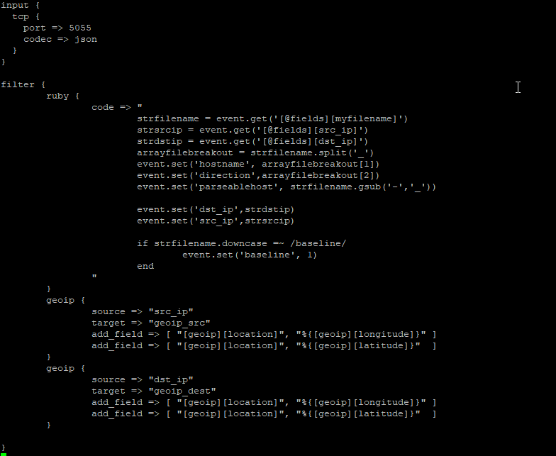
Next, the logstash pipeline needs to be configured to enrich log records with geoip information. There is a geoip filter available, which uses the MaxMind GeoIP database (this is refreshed automatically; currently, we do not merge in any geoip information for the private network address spaces) . You just need to indicate what field(s) have the IP address and where the location information should be stored. You can have multiple geographic IP fields – in this example, we map both source and destination IP addresses.
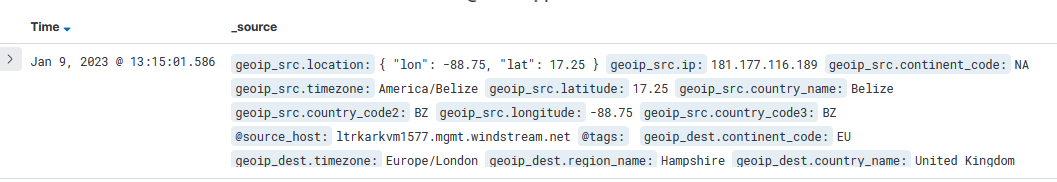
One logstash is restarted, the documents stored in Kibana will have geoip_src and geoip_dest fields:
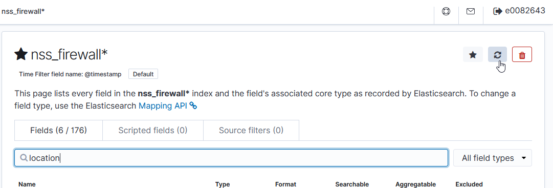
Once relevant data is being stored, use the refresh-looking button on the index pattern(s) to refresh the field list from stored data. This will add the geo-point items into the index pattern.
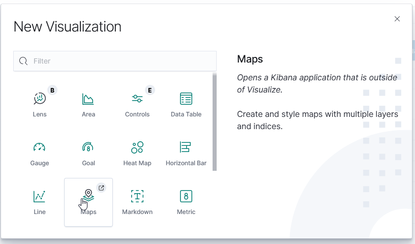
Once GeoIP information is available in the index pattern, select the “Maps” visualization
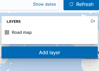
Leave the road map layer there (otherwise you won’t see the countries!)
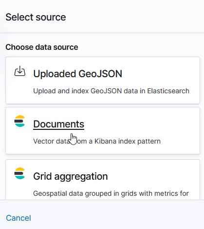
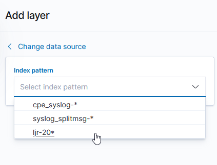
Select ‘Documents’ as the data source to link in ElasticSearch data
Select the index pattern that contains your data source (if your index pattern does not appear, then Kibana doesn’t recognize the pattern as containing geographic fields … I’ve had to delete and recreate my index pattern so the geographic fields were properly mapped).
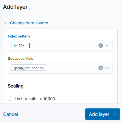
And select the field(s) that contain geographic details:
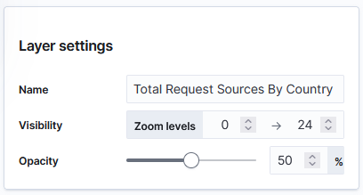
You can name the layer
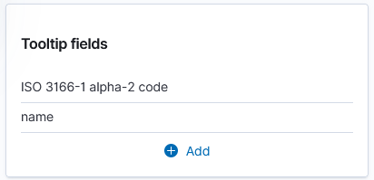
And add a tool tip that will include the country code or name
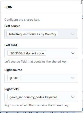
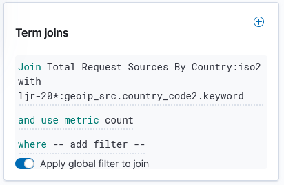
Under “Term joins”, add a new join. Click on “Join –select–” to link a field from the map to a field in your dataset.
In this case, I am joining the two-character country codes —
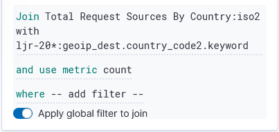
Normally, you can leave the “and use metric count” in place (the map is color coded by the number of requests coming from each country). If you want to add a filter, you can click the “where — add filter –” link to edit the filter.
In this example, I don’t want to filter the data, so I’ve left that at the default.
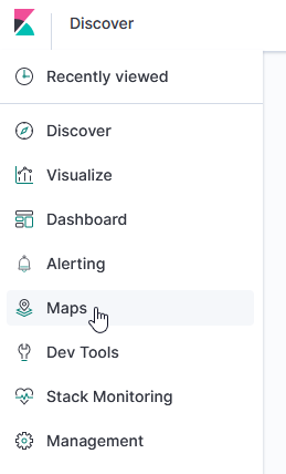
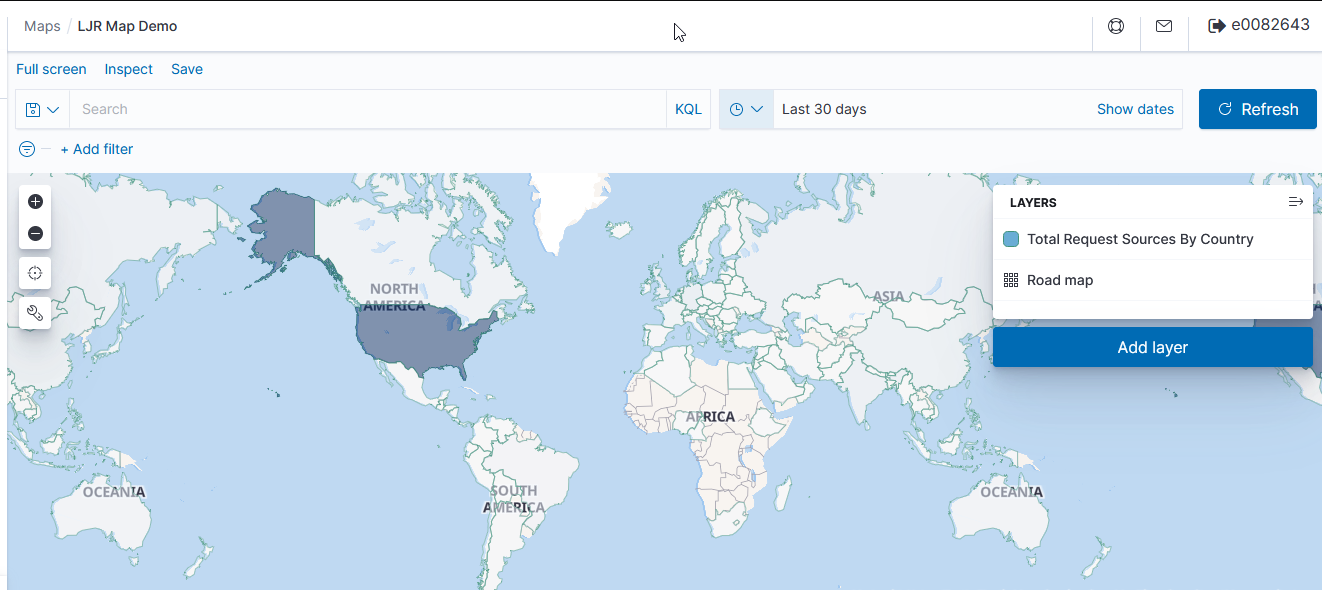
Click “Save & close” to save the changes to the map visualization. To view your map, you won’t find it under Visualizations – instead, click “Maps” along the left-hand navigation menu.
Voila – a map where the shading on a country gets darker the more requests have come from the country.
Internal Addresses
If we want to (and if we have information to map IP subnets to City/State/Zip/LatLong, etc), we can edit the database used for GeoIP mappings — https://github.com/maxmind/getting-started-with-mmdb provides a perl module that interacts with the database file. That isn’t currently done, so internal servers where traffic is sourced primarily from private address spaces won’t have particularly thrilling map data.
ElasticSearch, based on the Lucene search software, is a distributed search and analytics application which ingests, stores, and indexes data. Kibana is a web-based front-end providing user access to data stored within ElasticSearch.
What is OpenSearch?
In short, it’s the same but different. OpenSearch is also based on the Lucene search software, is designed to be a distributed search and analytics application, and ingests/stores/indexes data. If it’s essentially the same thing, why does OpenSearch exist? ElasticSearch was initially licensed under the open-source Apache 2.0 license – a rather permissive free software license. ElasticCo did not agree with how their software was being used by Amazon; and, in 2021, the license for ElasticSearch was changed to Server Side Public License (SSPL). One of the requirements of SSPL is that anyone who implements the software and sells their implementation as a service needs to publish their source code under the SSPL license – not just changes made to the original program but all other software a user would require to run the software-as-a-service environment for themselves. Amazon used ElasticSearch for their Amazon Elasticsearch Service offering, but was unable/unwilling to continue doing so under the new license terms. In April of 2021, Amazon Web Services created a fork of ElasticSearch as the basis for OpenSearch.
Differences Between OpenSearch and ElasticSearch
After the OpenSearch fork was created, the product roadmap for ElasticSearch was driven by ElasticCo and the roadmap for OpenSearch was community driven (with significant oversight and input from Amazon) – this means the products are not identical although they provide the same core functionality. Elastic publishes a list of features unique to ElasticSearch, and the underlying machine learning algorithms are different. However, the important components of the “unique” feature list have been implemented in OpenSearch over time.
The biggest differences are price and support. OpenSearch is free software – there is no purchasing a license to unlock features. It does appear that Amazon has an internal iteration of OpenSearch as their as-a-service offering provides features not available in the open-source OpenSearch code base, but that is only available for cloud customers. ElasticCo offers ElasticSearch as free software with a limited feature set. One critical limitation is user authentication mechanisms – we are unable to implement PingID as an authentication source with the free feature set. Advanced features not currently used today – machine learning based anomaly detection, as an example – are also unavailable in the free iteration of ElasticSearch. With an ElasticSearch license, we would also get vendor support. OpenSearch does not offer vendor support, although there are third party companies that will provide support services.
Both OpenSearch and ElasticSearch have community-based support forums available – I have gotten responses from developers on both forums for questions regarding usage nuances.
Salient Feature Comparison
Most companies have a list differentiating their product from the products offered by competitors – but the important thing is how the products differ as it relates to how an individual customer uses the product. A car that can have a fresh cup of espresso waiting for you as you leave for work might be amazing to some people, but those who don’t drink coffee won’t be nearly as impressed. So how do the two products compare for me?
Data ingestion – Data is ingested using the same mechanisms – ElasticCo’s filebeat and logstash are important components of data ingestion, and these components remain unchanged. This means existing processes that feed data into ElasticSearch today would not need to be changed to begin ingesting data into OpenSearch.
Data storage – Both products distribute searchable data over a cluster of servers. Data storage is “tiered” as hot, warm, and cold which allows less used data to reside on slower, less expensive resources. We have confirmed that ingested data is properly housed on cluster nodes designated for ‘hot’ storage and moved to ‘warm’ and ‘cold’ storage as dictated by defined policies. The item count to size ratio is similar between both products (i.e. storing ten million documents takes about the same amount of disk space). OpenSearch provides the ability to alert on transition failures (moving from hot to warm, for instance) which will reduce the amount of manual “health checking” required for the environment.
Search and aggregation – Both products allow both GUI and API searches of indexed data. Data can be aggregated as it is searched – returning the max/min/average value from a search, a count of records matching search criterion, creating sub-aggregations. ElasticSearch does have aggregations not available in OpenSearch, although these could be handled through custom scripted aggregations and many have corresponding GitHub issues requesting such an aggregation be added to OpenSearch (e.g. weighted average, geohash grid, or geotile grid)
auto-interval date histogram
x
categorize text
x
children
x
composite
x
frequent items
x
geohex grid
x
geotile grid
x
ip prefix
x
multi terms
x
parent
x
random sampler
x
rare terms
x
terms
x
variable width histogram
x
boxplot
x
geo-centroid
x
geo-line
x
median absolute deviation
x
rate
x
string stats
x
t-test
x
top metrics
x
weighted avg
x
Alerting – ElastAlert2 can be used to provide the same index monitoring and alerting functionality that ElastAlert currently provides with ElasticSearch. Additionally, OpenSearch includes a built-in alerting capability that might allow us to streamline the functionality into the base OpenSearch implementation.
API Access – Both ElasticSearch and OpenSearch provide API-based access to data. Queries to the ElasticSearch API endpoint returned expected data when directed to the OpenSearch API endpoint. The ElasticSearch python module can be used to access OpenSearch data, although there is a specific OpenSearch module as well.
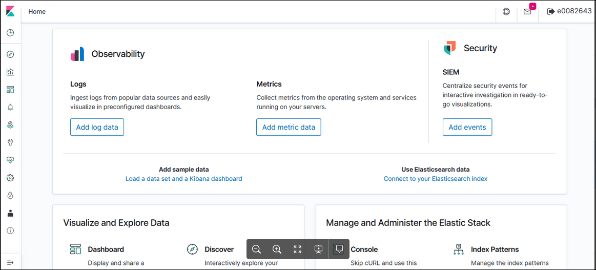
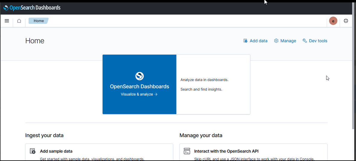
UX – ElasticSearch allows users to search and visualize data through Kibana; OpenSearch provides graphical user access in OpenSearch Dashboard. While the “look and feel” of the GUI differs (Kibana 8 looks different than the Kibana 7 we use today, too), the user functionality remains the same.
Kibana 7.7
OpenSearch Dashboards 2.2
Kibana uses “KQL” – Kibana Query Language – to compose searches while OpenSearch Dashboards uses “DQL” – Dashboards Query Language, but queries used in Kibana were used in OpenSearch Dashboard without modification.
Currently used visualizations are available in both Kibana and OpenSearch Dashboards
Kibana Visualization
OpenSearch Dashboards Visualization
But there are some currently unused visualizations that are unique to each product.
Area
x
x
Controls
x
x
Data Table
x
x
Gauge
x
x
Goal
x
x
Heat Map
x
x
Horizonal Bar
x
x
Lens
x
Line
x
x
Maps
x
Markdown
x
x
Metric
x
x
Pie
x
x
Tag Cloud
x
x
Timeline
x
x
TSVB
x
x
Vega
x
x
Vertical Bar
x
x
Coordinate Map
x
Gantt Chart
x
Region Map
x
Dashboards can be used to group visualizations.
Kibana
OpenSearch Dashboards
New features will be available in either OpenSearch or a licensed installation of ElasticSearch. Currently data is either retained as written or aged out of the system to save disk space. Either path allows us to roll up data – as an example retaining the total number of users per month or total bytes per month instead of retaining each detailed record. Additionally, we will be able to use the “anomaly detection” which is able to monitor large volumes of index data and highlight unusual events. Both newer ElasticSearch versions and OpenSearch offer a Tableau connector which may make data stored in the platform more accessible to users.
Sorry, again, Anya … I really mean it this time. Restart your ‘no posting about computer stuff’ timer!
I was able to cobble together a functional configuration to authenticate users through an OpenID identity provider. This approach combined the vendor documentation, ten different forum posts, and some debugging of my own. Which is to say … not immediately obvious.
Importantly, you can enable debug logging on just the authentication component. Trying to read through the logs when debug logging is set globally is unreasonable. To enable debug logging for JWT, add the following to config/log4j2.properties
On the OpenSearch servers, in ./config/opensearch.yml, make sure you have defined plugins.security.ssl.transport.truststore_filepath
While this configuration parameter is listed as optional, something needs to be in there for the OpenID stuff to work. I just linked the cacerts from our JDK installation into the config directory.
If needed, also configure the following additional parameters. Since I was using the cacerts truststore from our JDK, I was able to use the defaults.
plugins.security.ssl.transport.truststore_type
The type of the truststore file, JKS or PKCS12/PFX. Default is JKS.
plugins.security.ssl.transport.truststore_alias
Alias name. Optional. Default is all certificates.
Note that subject_key and role_key are not defined. When I had subject_key defined, all user logon attempts failed with the following error:
[2022-09-22T12:47:13,333][WARN ][c.a.d.a.h.j.AbstractHTTPJwtAuthenticator] [UOS-OpenSearch] Failed to get subject from JWT claims, check if subject_key 'userId' is correct.
[2022-09-22T12:47:13,333][ERROR][c.a.d.a.h.j.AbstractHTTPJwtAuthenticator] [UOS-OpenSearch] No subject found in JWT token
[2022-09-22T12:47:13,333][WARN ][o.o.s.h.HTTPBasicAuthenticator] [UOS-OpenSearch] No 'Basic Authorization' header, send 401 and 'WWW-Authenticate Basic'
Finally, use securityadmin.sh to load the configuration into the cluster:
Restart OpenSearch and OpenSearch Dashboard — in the role mappings, add custom objects for the external user IDs.
When logging into the Dashboard server, users will be redirected to the identity provider for authentication. In our sandbox, we have two Dashboard servers — one for general users which is configured for external authentication and a second for locally authenticated users.
There’s often a difference between hypothetical (e.g. the physics formula answer) and real results — sometimes this is because sciences will ignore “negligible” factors that can be, well, more than negligible, sometimes this is because the “real world” isn’t perfect. In transmission media, this difference is a measurable “loss” — hypothetically, we know we could send X data in Y delta-time, but we only sent X’. Loss also happens because stuff breaks — metal corrodes, critters nest in fiber junction boxes, dirt builds up on a dish. And it’s not easy, when looking at loss data at a single point in time, to identify what’s normal loss and what’s a problem.
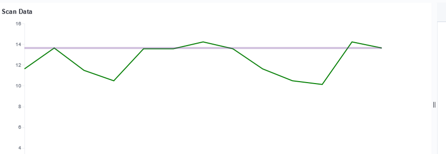
We’re starting a project to record a baseline of loss for all sorts of things — this will allow individuals to check the current loss data against that which engineers say “this is as good as it’s gonna get”. If the current value is close … there’s not a problem. If there’s a big difference … someone needs to go fix something.
Unfortunately, creating a graph in Kibana that shows the baseline was … not trivial. There is a rule mark that allows you to draw a straight line between two points. You cannot just say “draw a line at y from 0 to some large value that’s going to be off the graph. The line doesn’t render (say, 0 => today or the year 2525). You cannot just get the max value of the axis.
I finally stumbled across a series of data contortions that make the baseline graphable.
The data sets I have available have a datetime object (when we measured this loss) and a loss value. For scans, there may be lots of scans for a single device. For baselines, there will only be one record.
The joinaggregate transformation method — which appends the value to each element of the data set — was essential because I needed to know the largest datetime value that would appear in the chart.
The lookup transformation method — which can access elements from other data sets — allowed me to get that maximum timestamp value into the baseline data set. Except … lookup needs an exact match in the search field. Luckily, it does return a random (I presume either first or last … but it didn’t matter in this case because all records have the same max date value) record when multiple matches are found.
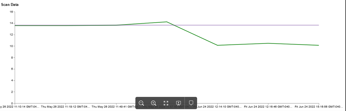
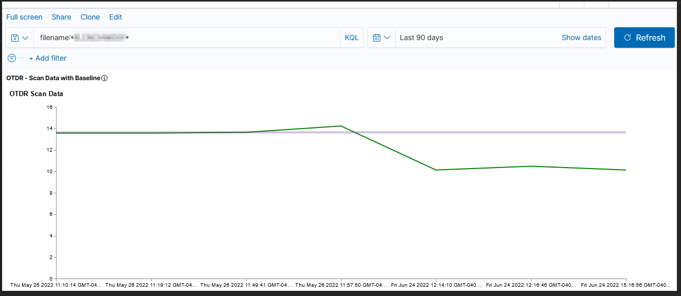
Voila — a chart with a horizontal line at the baseline loss value. Yes, I randomly copied a record to use as the baseline and selected the wrong one (why some scans are below the “good as it’s ever going to get” baseline value!). But … once we have live data coming into the system, we’ll have reasonable looking graphs.
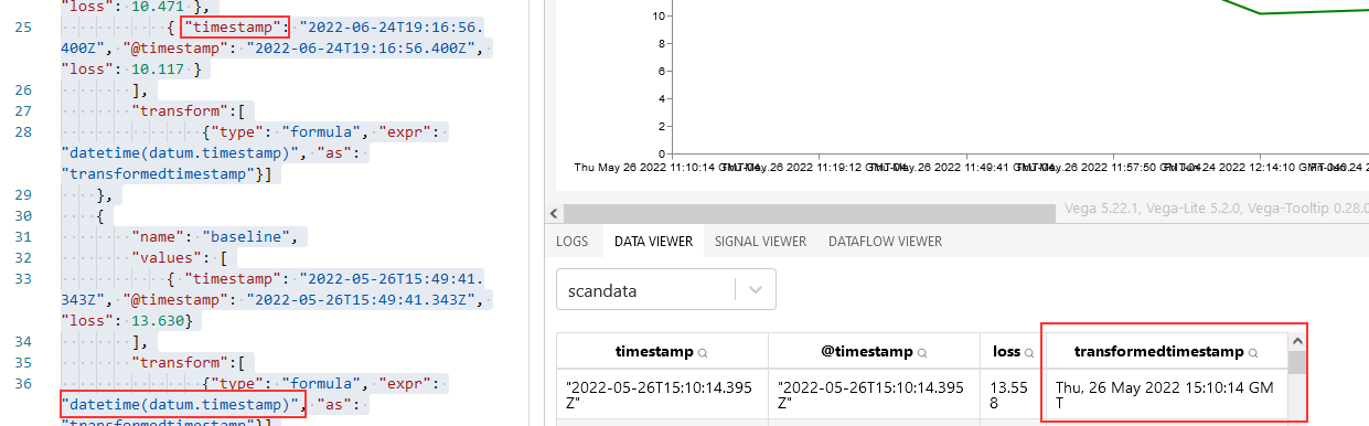
We have data created by an external source (i.e. I cannot just change the names used so it works) — the datetime field is named @timestamp and I had an awful time figuring out out how to address that element within a transformation expression.
Just to make sure I wasn’t doing something silly, I created a copy of the data element named without the at symbol. Voila – transformedtimestamp is populated with a datetime element.
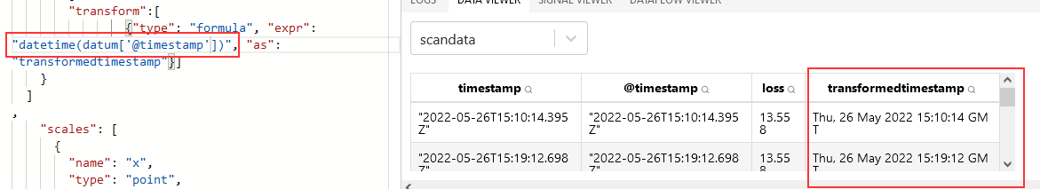
I finally figured it out – it appears that I have encountered a JavaScript limitation. Instead of using the dot-notation to access the element, the array subscript method works – not datum.@timestamp in any iteration or with any combination of escapes.
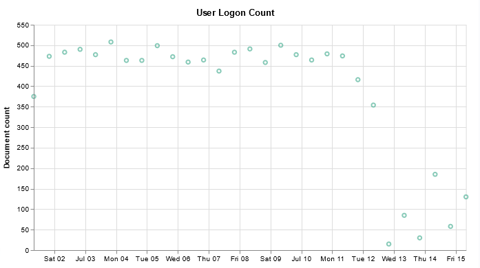
I have finally managed to produce a chart that includes a query — I don’t want to have to walk all of the help desk users through setting up the query, although I figured having the ability to select your own time range would be useful.
{
  $schema: https://vega.github.io/schema/vega-lite/v2.json
  title: User Logon Count

  // Define the data source
  data: {
    url: {
      // Which index to search
      index: firewall_logs*

      body: {
        _source: ['@timestamp', 'user', 'action']

"query": {
	"bool": {
		"must": [{
				"query_string": {
					"default_field": "subtype",
					"query": "user"
				}
			},
	   {
				"range": {
					"@timestamp": {
						"%timefilter%": true
                    			}
                  		}
     	}]
	}
}


        aggs: {
          time_buckets: {
            date_histogram: {
              field: @timestamp
              interval: {%autointerval%: true}
              extended_bounds: {
                // Use the current time range's start and end
                min: {%timefilter%: "min"}
                max: {%timefilter%: "max"}
              }
              // Use this for linear (e.g. line, area) graphs.  Without it, empty buckets will not show up
              min_doc_count: 0
            }
          }
        }
        size: 0
      }
    }
    format: {property: "aggregations.time_buckets.buckets"}
  }
  mark: point
  encoding: {
    x: {
      field: key
      type: temporal
      axis: {title: false} // Don't add title to x-axis
    }
    y: {
      field: doc_count
      type: quantitative
      axis: {title: "Document count"}
    }
  }
}
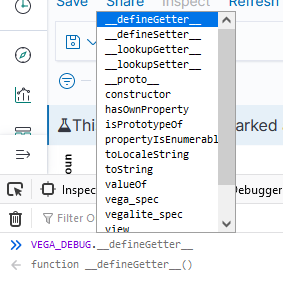
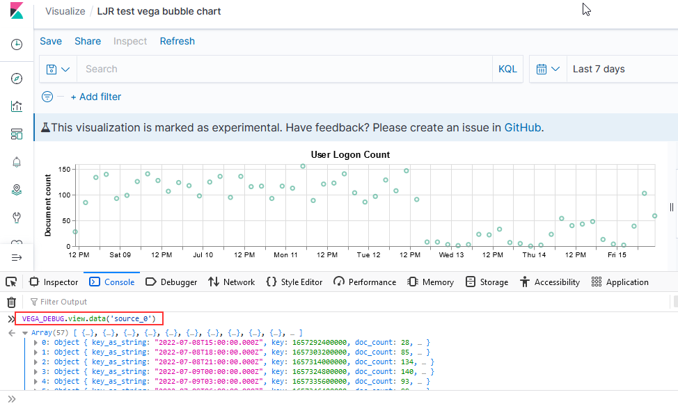
If you open the browser’s developer console, you can access debugging information. This works when you are editing a visualization as well as when you are viewing one. To see a list of available functions, type VEGA_DEBUG. and a drop-down will show you what’s available. The command “VEGA_DEBUG.vega_spec” outputs pretty much everything about the chart.
To access the data set being graphed with the Vega Lite grammar, use “VEGA_DEBUG.view.data(“source_0)” — if you are using the Vega grammar, use the dataset name that you have defined.
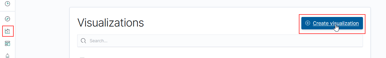
To create a new visualization, select the visualization icon from the left-hand navigation menu and click “Create visualization”. You’ll need to select the type of visualization you want to create.
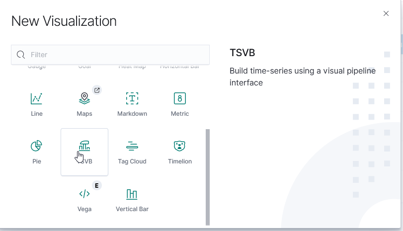
TSVB (Time Series Visualization Builder)
The Time Series Visualization Pipeline is a GUI visualization builder to create graphs from time series data. This means the x-axis will be datetime values and the y-axis will the data you want to visualize over the time period. To create a new visualization of this type, select “TSVB” on the “New Visualization” menu.
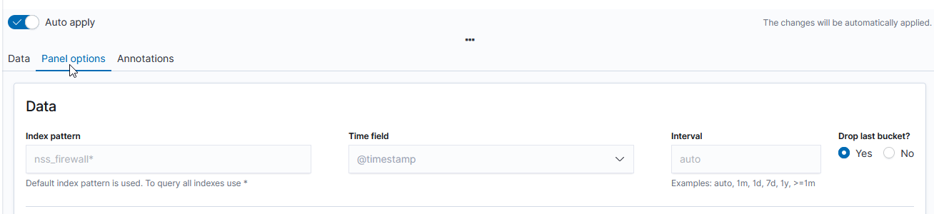
Scroll down and select “Panel options” – here you specify the index you want to visualize. Select the field that will be used as the time for each document (e.g. if your document has a special field like eventOccuredAt, you’d select that here). I generally leave the time interval at ‘auto’ – although you might specifically want to present a daily or hourly report.
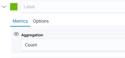
Once you have selected the index, return to the “Data” tab. First, select the type of aggregation you want to use. In this example, we are showing the number of documents for a variety of policies.
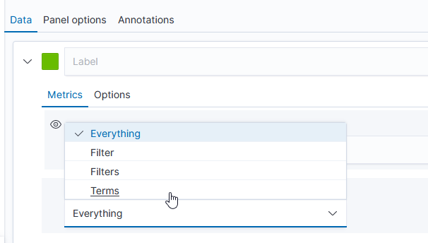
The “Group by” dropdown allows you to have chart lines for different categories (instead of just having the count of documents over the time series, which is what “Everything” produces) – to use document data to create the groupings, select “Terms”.
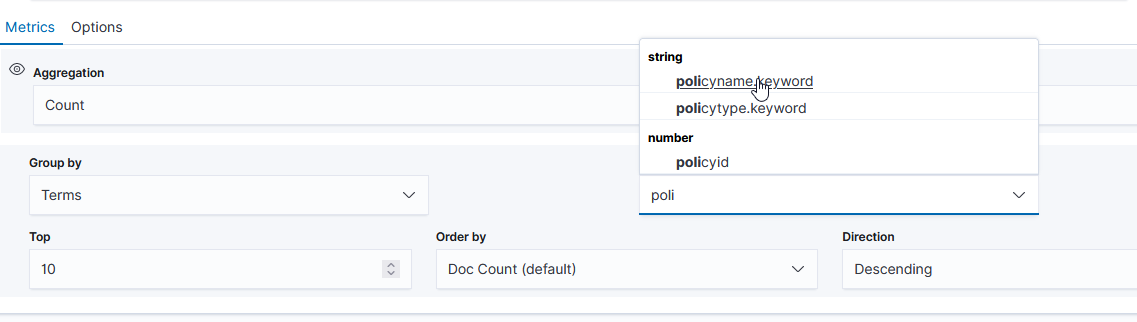
Select the field you want to group on – in this case, I want the count for each unique “policyname” value, so I selected “policyname.keyword” as the grouping term.
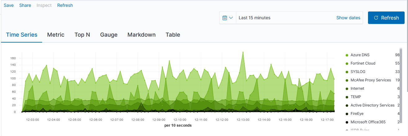
Voila – a time series chart showing how many documents are found for each policy name. Click “Save” at the top left of the chart to save the visualization.
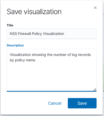
Provide a name for the visualization, write a brief description, and click “Save”. The visualization will now be available for others to view or for inclusion in dashboards.
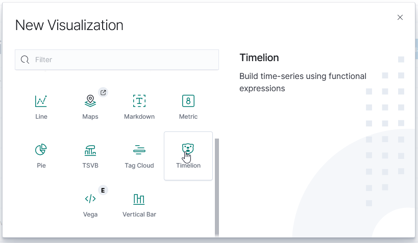
TimeLion
TimeLion looks like it is going away soon, but it’s what I’ve seen as the recommendation for drawing horizontal lines on charts.
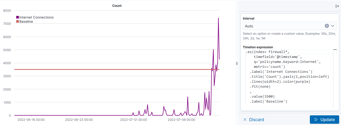
This visualization type is a little cryptic – you need to enter Timelion expression — .es() retrieves data from ElasticSearch, .value(3500) draws a horizontal line at 3,500
If there is null data at a time value, TimeLion will draw a discontinuous line. You can modify this behavior by specifying a fit function.
Note that you’ll need to click “Update” to update the chart before you are able to save the visualization.
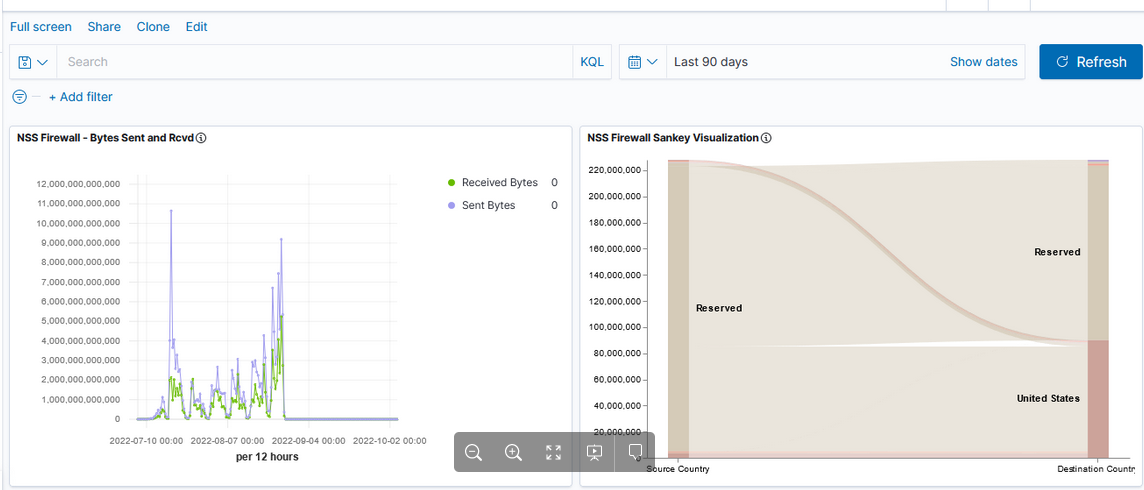
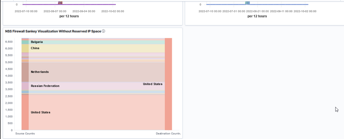
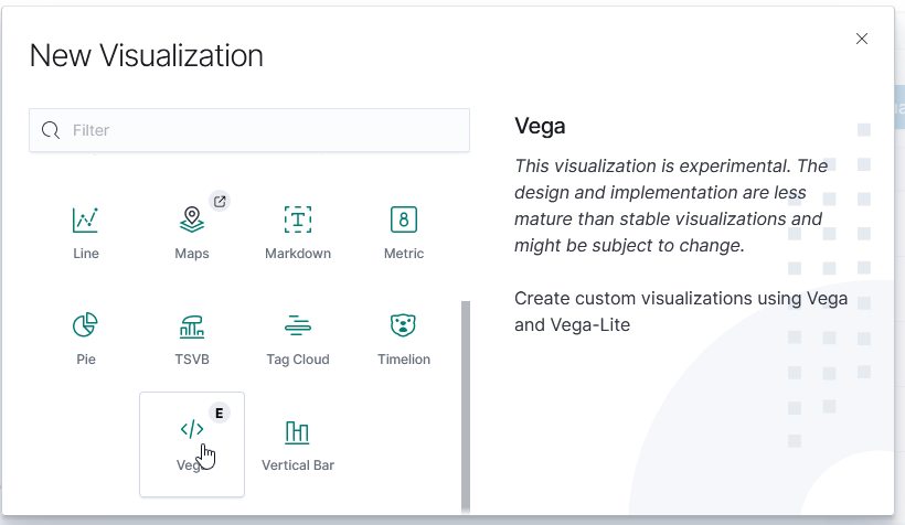
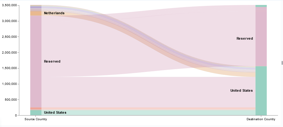
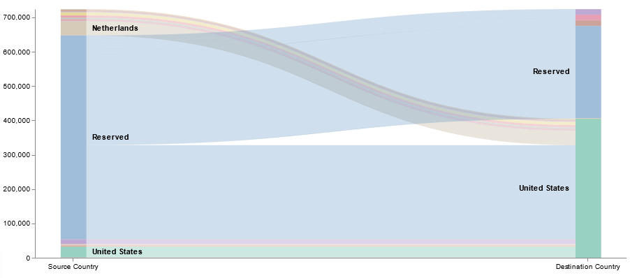
Now that we’ve got a lot of data being ingested into our ELK platform, I am beginning to build out visualizations and dashboards. This Vega visualization (source below) shows the number of connections between source and destination countries.