The following formula prints just the substring found before the first dash from the data in cell A2:
=LEFT(A2, FIND("-", A2) - 1)
The following formula prints just the substring found before the first dash from the data in cell A2:
=LEFT(A2, FIND("-", A2) - 1)
In case anyone else has been low-key bothered by the fact their Excel formula bar seems to have turned into a strange monospace font — you can change the default font around & that impacts the formula bar. Arial looks fairly reasonable for me. But there are lots of other fonts to chose from!
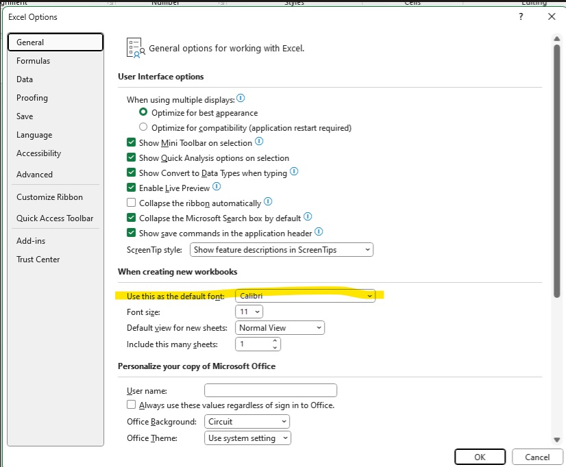
Also looks like a future update will include an option to not use monospace fonts for formulae … https://techcommunity.microsoft.com/blog/excelblog/excel’s-formula-bar-gets-a-new-look/3902462
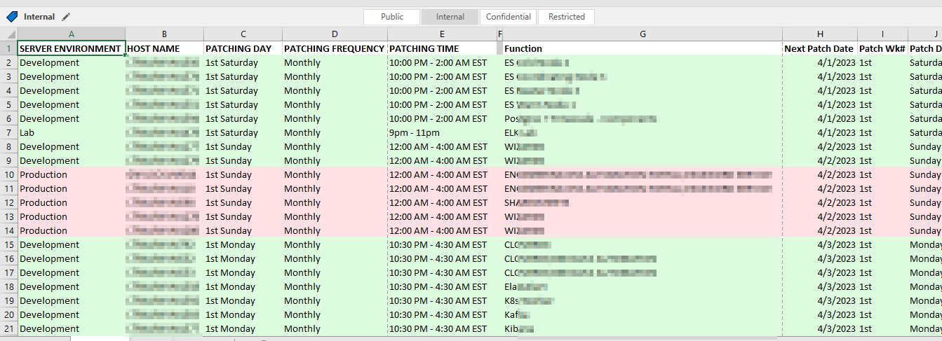
Our patching schedules are algorithmic – the 1st Tuesday of the month, the 3rd Wednesday of the month, etc. But that’s not particularly useful for notifying end users or for us to verify functionality after patching.
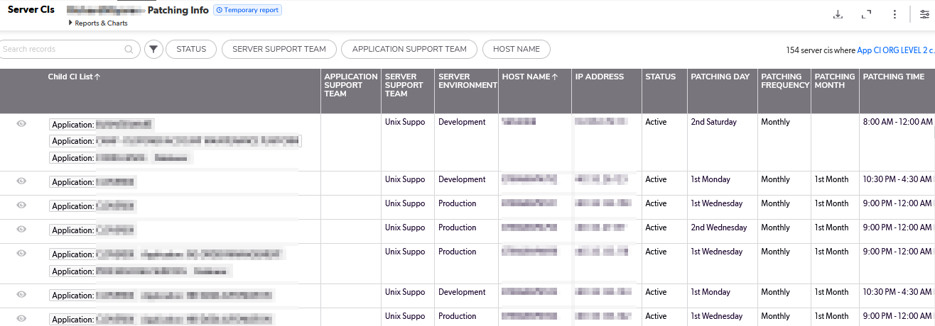
Long term, I think we can pull the source data from a database and create appointment items each month for whatever list of servers will be patched that month based on a relative date (so no one has to add new servers or remove decommissioned servers). But, short term? I really wanted a way to see what date a server would be patched. So I created a but of a convoluted spreadsheet to produce this information based on a list of servers and patching schedule patterns.
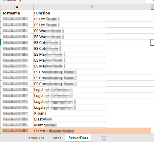
There are two “extra” tabs used – “Dates” used to say what month and year I want the patching dates for
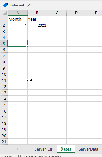
And “ServerData” which provides a cross-reference between the server names and a useful description.
There are then a series of formulae used to add columns to our source data. First, the “Function” is populated in column G with a VLOOKUP =VLOOKUP(B2,ServerData!A:B,2,FALSE)
Columns I and J break the “1st Saturday” into the two components – week of month and day of week –
I =LEFT(C2,3)
J =RIGHT(C2,LEN(C2)-4)
Columns K and L then map these components into numeric values I can use in a formula:
K =IF(I2=”1st”,1,IF(I2=”2nd”,2,IF(I2=”3rd”,3,IF(I2=”4th”,4,”Unscheduled”))))
L =IF(J2=”Sunday”,1,IF(J2=”Monday”,2,IF(J2=”Tuesday”,3,IF(J2=”Wednesday”,4,IF(J2=”Thursday”,5,IF(J2=”Friday”,6,IF(J2=”Saturday”,7,”Unscheduled”)))))))
And finally a formula in column H that turns the week of month and day of week values into an actual date within the month and year on the “Dates” tab:
H =DATE(Dates!$B$2,Dates!$A$2,1+7*K2)-WEEKDAY(DATE(Dates!$B$2,Dates!$A$2,8-L2))
Voila – I have a spreadsheet that says we should expect to see this specific list of servers being patched tonight.
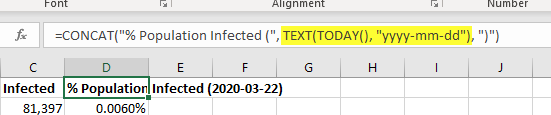
Here’s a trick to include the current date in an Excel string — especially useful if you want to include the current date on a graph without having to actually type the current date each time. If you just include TODAY(), you get the integer representation. Wrap TODAY() in TEXT() and supply the formatting you want (“yyyy-mm-dd” in my example). Voila, a date like 2020-03-22 instead of 43912.
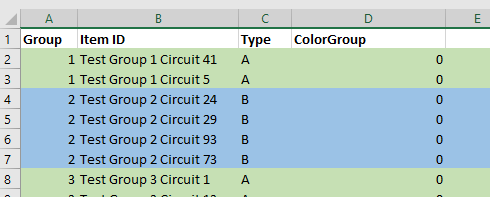
I need to programmatically parse an Excel file where items are grouped with arbitrary group sizes. We don’t want the person filling out the spreadsheet to need to fill in a group # column … so I’m exploring ways to read cell formatting so something like color can be used to show the groups. Reading the formatting isn’t a straight-forward process, so I wondered if Excel could populate a group number cell based on the cell’s attributes.
While it is possible, it’s not a viable solution. The mechanism to access data about a cell cannot be accessed directly and, unfortunately, requires a macro-enabled workbook. The mechanism also requires the user to remember to update the spreadsheet calculations when they have finished colorizing the rows. While I won’t be using this approach in my current project … I thought I’d record what I did for future reference.
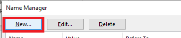
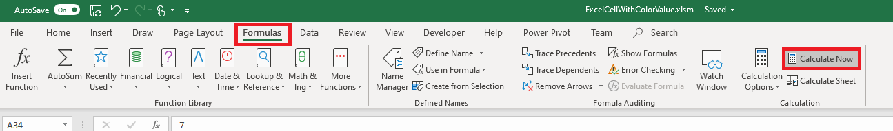
We need to define a ‘name’ for the function. On the “Formulas” tab, select “Name Manager”.
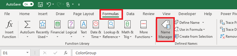
Select ‘New’
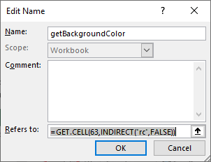
Provide a name – I am using getBackgroundColor – and put the following in the “refers to” section: =GET.CELL(63,INDIRECT(“rc”,FALSE))
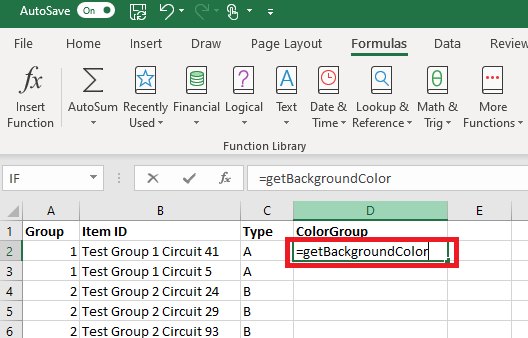
Now we can use this name within the cell formula:
Select the rows for your first group and change the “fill color” of the row.
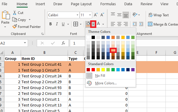
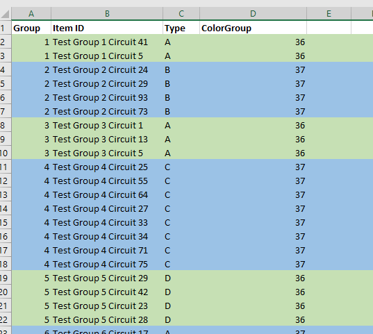
Repeat this process to colorize all of your groups – you can re-use a color as long as adjacent groups have different colors. Notice that the “ColorGroup” values do not change when you colorize your groups.
On the “Forumlas” tab, select “Calculate Now”
Now the colorized cells will have a non-zero value.
As we are upgrading groups to Microsoft Teams, we need to be able to identify which activities need to be performed each week. While highlighting today’s date is a start, it is better to identify which tasks need to be performed in the upcoming week so we can plan ahead.
To accomplish this, I use a conditional formatting rule. It highlights all of the date values that fall between today and seven days in the future. How? In conditional formatting, you can use a formula to determine which cells to format. My selection rage is E2 through J20, so the conditional formatting formula is based off of the E2 cell.
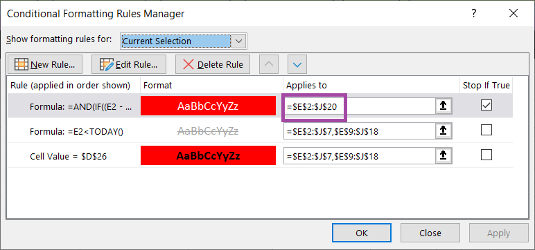
The formula AND’s to IF functions. If the difference between the cell date and today is less than 8 (less than 8 days in the future) AND if the difference between the cell date and today is greater than or equal to zero (today or a future date), the rule evaluates to TRUE and the highlighting is applied.
=AND(IF((E2 – TODAY()) <8,1,0),IF((E2 – TODAY()) >= 0,1,0))
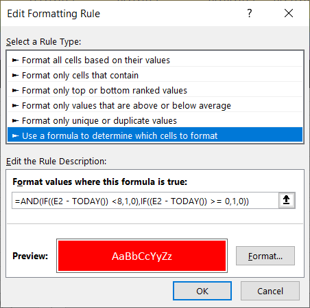
The result – every activity we need to plan for in the upcoming week is highlighted.
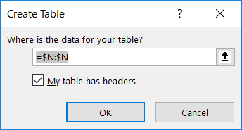
Remove duplicates is a quick way to obtain a unique list of records; every time the source data is updated, though, you’ve got to copy and ‘remove duplicates’ again. There’s a better way! Use Power Query to create a unique list that can be updated with a single click.
To use Power Query, first highlight the column containing the information for which you want a list of unique values.
On the “Data” ribbon bar, select “From Table/Range”
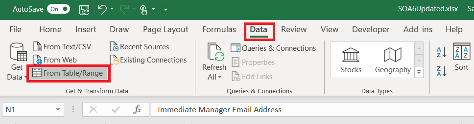
You’ll be asked to confirm where the source data is located – the highlighted selection should appear. Click “OK” to continue.
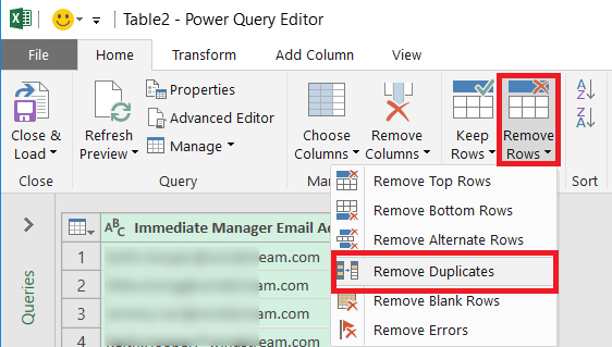
A new window will open – the Power Query Editor. On the “Home” ribbon bar, click on “Remove Rows” and select “Remove Duplicates”
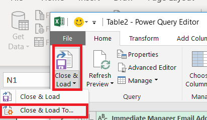
A unique list of values has been extracted in the Power Query editor – but you want to insert that data into your spreadsheet. Click the drop-down by “Close & Load” then select “Close & Load To …”
Now you can select where you want your list of unique values to appear – I am creating a table in an existing worksheet. Click “OK” to insert the unique list.
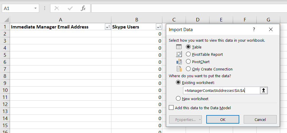
Voila, I now have a unique list.
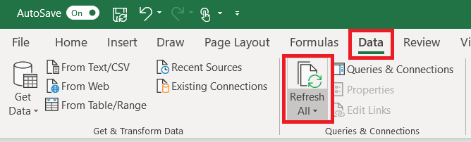
What happens when new records are added to my source data? The Power Query table does not automatically update as values are added to the source data. On the “Data” ribbon bar, click “Refresh All” to update the unique value list.
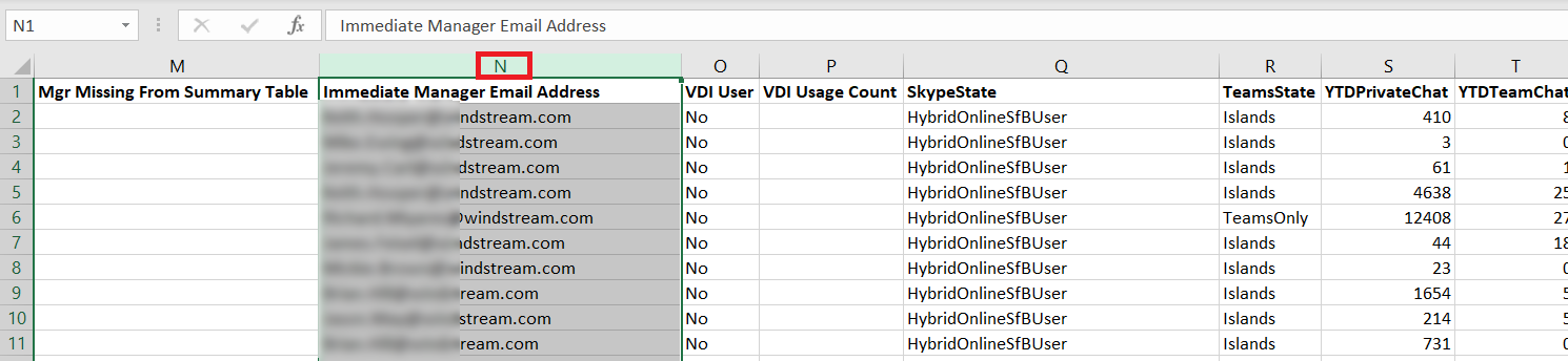
I mentioned yesterday that we’re creating groups based on the upper level manager through whom individuals report. Since my groups are based on the upper level managers, I need to be able to identify when a new individual pops into the list of upper level managers. Real upper level management doesn’t change frequently, but unfilled positions create gaps in the reporting structure. I call the manager before the gap the highest-ranking person in that vertical and that individual’s reporting subtree becomes a group.
Determining if values from one list appear in another list is easy in Microsoft Access – it’s an unmatched query. I’d rather not have to switch between the two programs, and I was certain an Excel formula could do the same thing. It can!
The formula is:
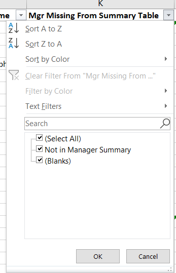
=IF(ISNA(VLOOKUP(H2,SOA6MgrSummary!A:A,1,FALSE)),”Not in Manager Summary”,””)
And it does flag any manager from column H that does not appear in my list of upper level managers.

I am also able to filter my spreadsheet to display only records where the upper level manager does not appear in my summary table.
What is my formula doing? It is a combination of three functions
=IF(ISNA(VLOOKUP(H2,SOA6MgrSummary!A:A,1,FALSE)),”Not in Manager Summary”,””)
It starts with the IF function – a logical comparison – which is used as if(Test,ResultIfTestIsTrue, ResultIfTestIsFalse).
If the test is true, “Not in Manager Summary” will be put into the cell. If the test is false, nothing (“”) will be put into the cell.
The test itself is two functions. I’ve documented the VLOOKUP function previously, but briefly it searches a range of data for a specific value. If the value is found, it returns something. If the value isn’t found, it returns N/A.
In conjunction with the VLOOKUP, I am using the ISNA function. This function is a logic test – it returns TRUE when the value is N/A and FALSE otherwise.
So my formula says “Look for the value of cell H2 in column A of the SOA6MgrSummary tab. If the result is N/A, put ‘Not in Manager Summary’ in this cell, otherwise leave this cell empty”.
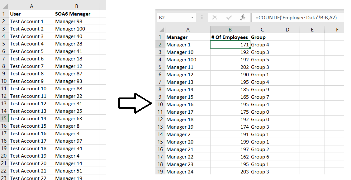
For a project, we need to divide the entire company into groups. I chose organizational structure because it’s easy – I can determine the reporting structure for any employee or contractor, and I can roll people into groups under which ever level of manager I want.
The point of making groups, though, is to have close to the same number of people in each group. While I can use COUNTIFS to count the number of people who report up through each manager, I need to add those totals for each group of managers to determine how many individuals fall in each group. How many employees are included in Group 0?
This is actually quite easy – just like count has a conditional counterpart, countifs, sum has a conditional counterpart sumifs
The usage is =SUMIFS( Range Of Data To Sum, Range Of Data Where Criterion Needs To Match, Criterion That Needs To Match)
You can use multiple criteria ranges and corresponding criteria in your conditional sum — =SUMIFS(SumRange,CriterionRange1,CriterionMatch1,CriterionRange2,CriterionMatch2,…,CriterionRangeN,CriterionMatchN).
I only have one condition, so with a quick listing of the groups, I can add a column that tells me how many individuals are included in each group.
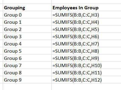
Bonus did you know – instead of specifying a start and end cell for a range, you can use the entire column. Instead of saying my “Range of data to sum” is B2:B101, I just used B:B to select the entire “B” column.
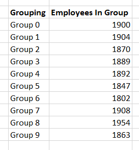
Viewing the values, I can see that my group size is not consistent.
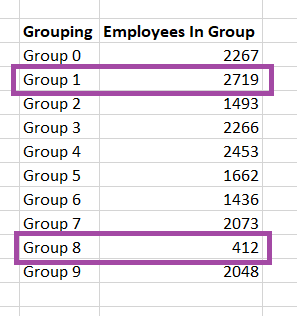
As I adjust the group to which the manager is assigned, these sums are updated in real-time.
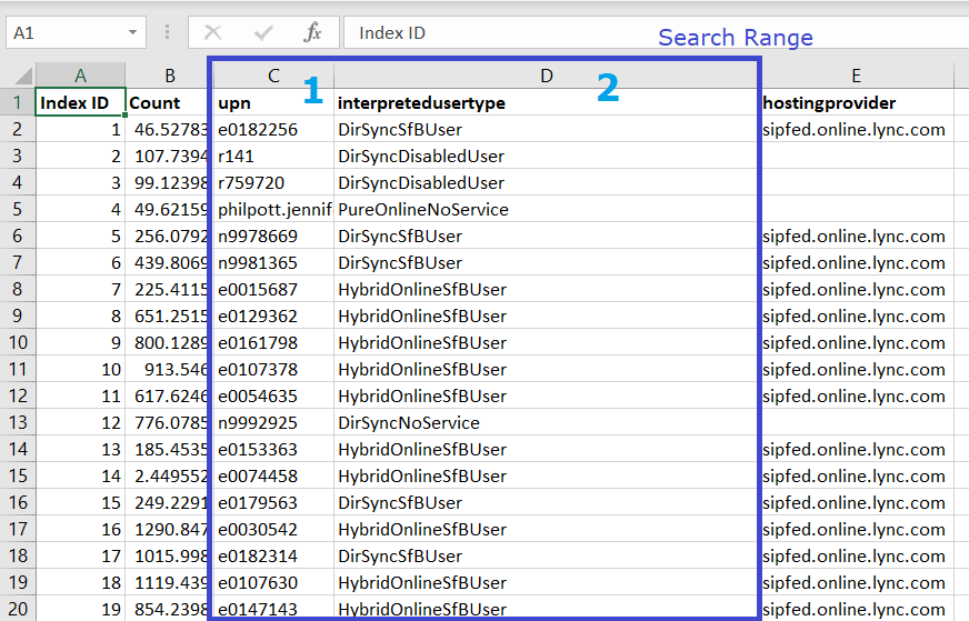
I frequently need to correlate two sets of data – generally information about accounts, where the logon ID will be found in both data sets. I’ve imported my information into Access, defined a relationship between the two tables, and used a query to correlate my data. I’ve written quick scripts to pull the data into an associative array for correlation. These are not quick approaches.
Using the VLOOKUP function in Excel, you can search through data in rows and retrieve values from the record’s other columns. HLOOKUP provides the same function, but searches data in columns and retrieves values from the record’s other rows (Vertical Lookup and Horizontal Lookup).
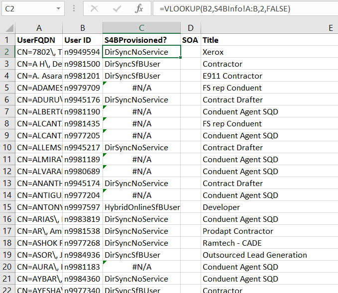
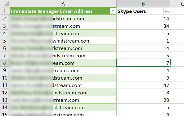
Today, I have a list of individuals with their reporting structure and need to identify which accounts have Skype for Business provisioned.
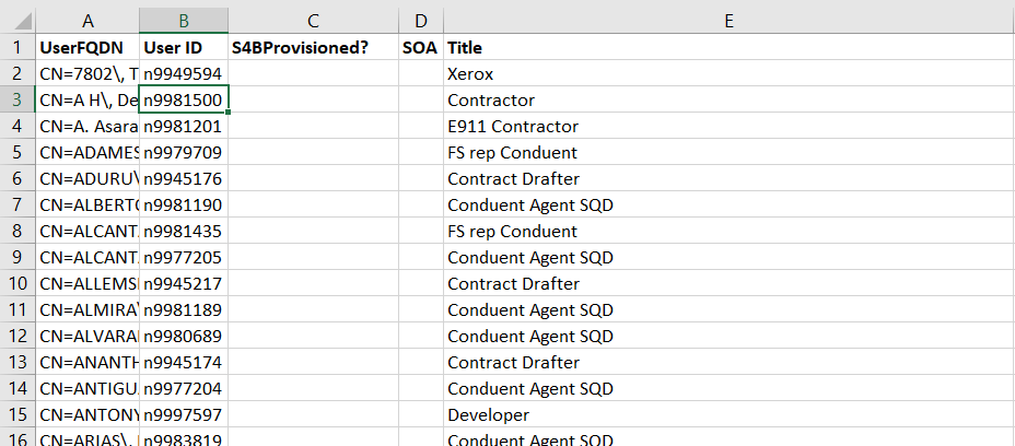
The Skype user list is, unfortunately, comes from a different program.
To lookup user IDs from the first table against the Skype info in the second table, I use =VLOOKUP(B2,S4BInfo!A:B,2,FALSE)
The first parameter in the function is the information you want to find, the second parameter is the area where you’ll be looking for the data, the third parameter is the column in that range that you want to return when a match is found. The fourth parameter indicates if you want to find the closest match (‘TRUE’) or an exact match (‘FALSE’). So my formula says “find the value in B2 within columns A and B of the SBInfo tab. Return the value from column 2 of that range, and I want an identical match”.
Note that the third parameter column number may not match the column number in the sheet – if I used the range C:D from the table below, I would still want to return the data in column 2 because my target data is still the second column in the search range.
Fill down and I have a single table that contains both the reporting information that I needed and a column indicating if the individual has a Skype for Business account