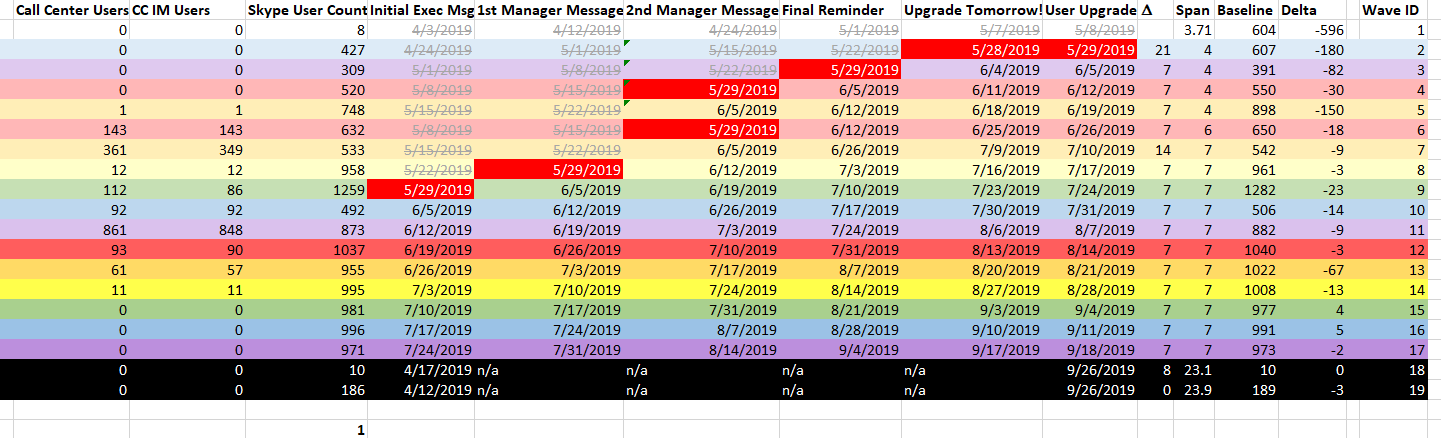
As we are upgrading groups to Microsoft Teams, we need to be able to identify which activities need to be performed each week. While highlighting today’s date is a start, it is better to identify which tasks need to be performed in the upcoming week so we can plan ahead.

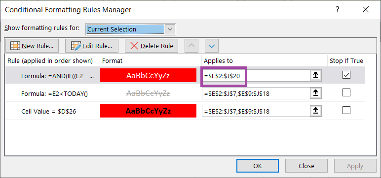
To accomplish this, I use a conditional formatting rule. It highlights all of the date values that fall between today and seven days in the future. How? In conditional formatting, you can use a formula to determine which cells to format. My selection rage is E2 through J20, so the conditional formatting formula is based off of the E2 cell.

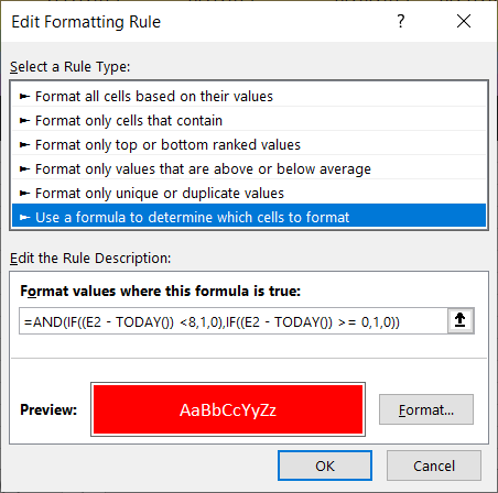
The formula AND’s to IF functions. If the difference between the cell date and today is less than 8 (less than 8 days in the future) AND if the difference between the cell date and today is greater than or equal to zero (today or a future date), the rule evaluates to TRUE and the highlighting is applied.

=AND(IF((E2 – TODAY()) <8,1,0),IF((E2 – TODAY()) >= 0,1,0))

The result – every activity we need to plan for in the upcoming week is highlighted.