Remove duplicates is a quick way to obtain a unique list of records; every time the source data is updated, though, you’ve got to copy and ‘remove duplicates’ again. There’s a better way! Use Power Query to create a unique list that can be updated with a single click.

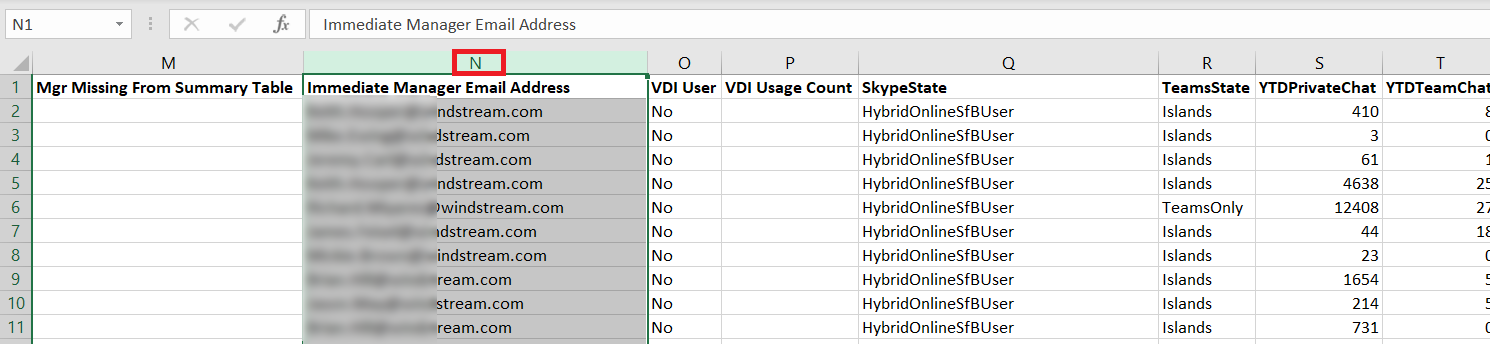
To use Power Query, first highlight the column containing the information for which you want a list of unique values.

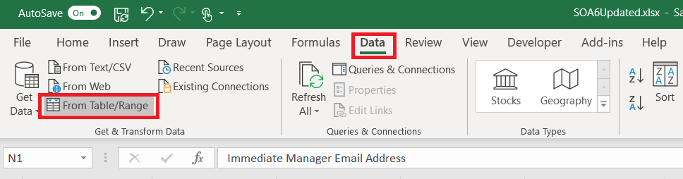
On the “Data” ribbon bar, select “From Table/Range”

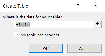
You’ll be asked to confirm where the source data is located – the highlighted selection should appear. Click “OK” to continue.

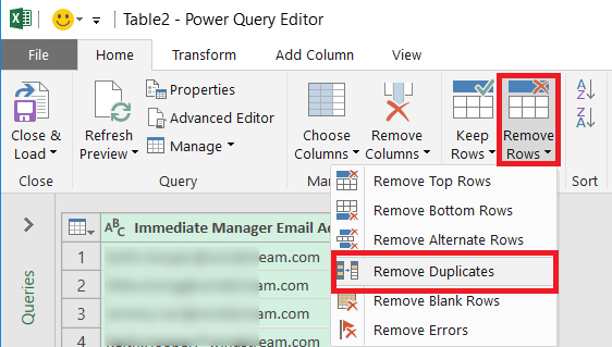
A new window will open – the Power Query Editor. On the “Home” ribbon bar, click on “Remove Rows” and select “Remove Duplicates”

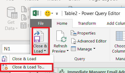
A unique list of values has been extracted in the Power Query editor – but you want to insert that data into your spreadsheet. Click the drop-down by “Close & Load” then select “Close & Load To …”

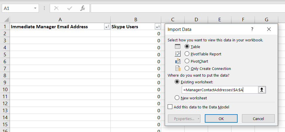
Now you can select where you want your list of unique values to appear – I am creating a table in an existing worksheet. Click “OK” to insert the unique list.

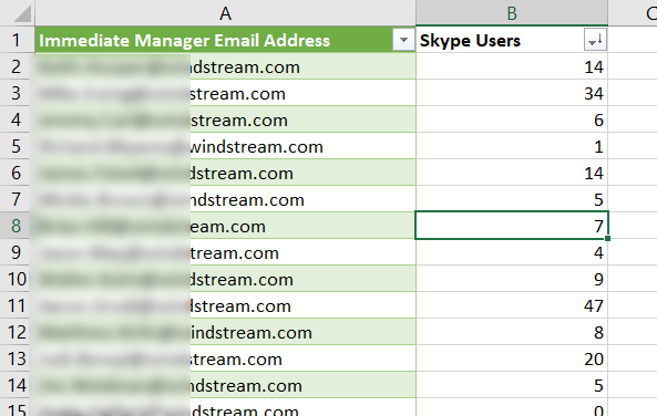
Voila, I now have a unique list.

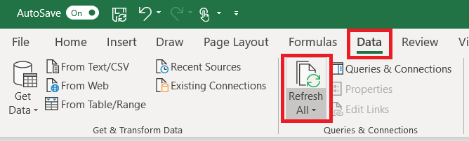
What happens when new records are added to my source data? The Power Query table does not automatically update as values are added to the source data. On the “Data” ribbon bar, click “Refresh All” to update the unique value list.