Category: Database

Using Graph Database to Track Plant Hybridization

Graph databases are designed to both store data and record relationships between data elements. I wondered if this would be useful in tracking cross-breeding projects – essentially building “family trees” of the entity being cross-bred. The data model would have nodes with the hybrid with notes on it. Relationships for PARENT_M and PARENT_F (male and female parent of the hybrid) would be used to associate nodes.

Graph databases have a concept of pathing – what nodes do we need to traverse to get from A to B – but to create a lineage for the plants, you need to know the starting point. Which is great if you want to play six degrees of separation and find a path between two known people, but not great if I just want to know what the lineage is of Tomato #198. To make pathing possible, I needed to add a common root node to all of heirloom seedstocks – PLANT0

This allows me to take any plant and find the paths from PLANT0 to it

MATCH
p=(Tomato0:TOMATO {name: 'PLANT0'})-[*]->(Tomato8:TOMATO{name: 'Tomato0000008'})
RETURN p

And visualize the genetic heritage of the hybrid.


Neo4J — Setting Up and Basic Record Management

Setting up a Neo4J Database

Ostensibly, you can create a new database using “create database somethingorother”. However, that is if you are using the enterprise edition. Running the community edition, you can only run one database. Attempting to create a new database will produce an error indicating Neo.ClientError.Statement.UnsupportedAdministrationCommand

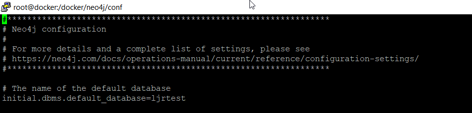
To use a database with a custom name, I need to edit neo4j.conf and set initial.dbms.default_database

Then create a Docker container – I am mapping /data to an external directory to persist my data and /var/lib/neo4j/conf to an external directory to persist configuration

docker run -dit --name neo4j --publish=7474:7474 --publish=7687:7687 --env=NEO4J_AUTH=none --volume=/docker/neo4j/data:/data --volume=/docker/neo4j/conf:/var/lib/neo4j/conf neo4j

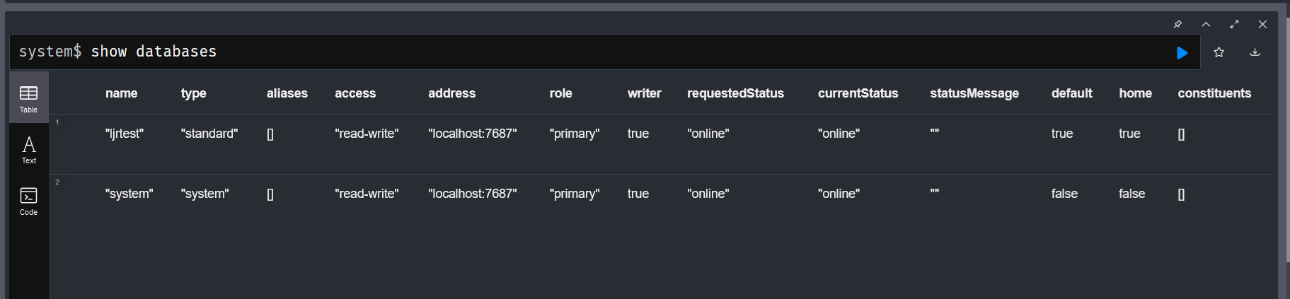
Listing the databases using “show databases” will show my custom database name

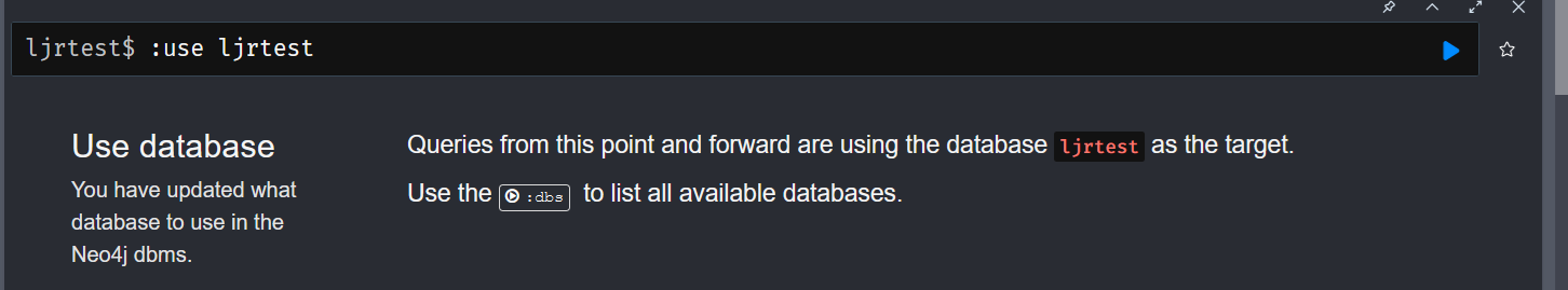
Switch to our database with the “:use” instruction
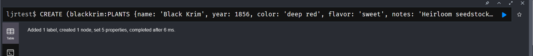
Create single nodes

CREATE (:PLANTS {name: ‘Black Krim’, year: 1856, color: ‘deep red’, flavor: ‘sweet’, notes: ‘Heirloom seedstock’})

Note: After I started using my data, I realized that “PLANTS” is a silly label to use since they will all be plants. I recreated all of my data with nodes labeled “TOMATO” so I can also track peppers, daffodils, and any other plants we start hybridizing.

Load of all records:

CREATE(:TOMATO {flavor: "air",notes: "hypothetical",color: "invisible",year: "1",name: "PLANT0"});
CREATE(:TOMATO {flavor: "acidic",notes: "Heirloom seedstock",color: "purple",year: 1890,name: "Cherokee Purple"});
CREATE(:TOMATO {flavor: "sweet",notes: "Heirloom seedstock",color: "bright red",name: "Whittemore"});
CREATE(:TOMATO {flavor: "sweet",notes: "Heirloom seedstock",color: "deep red",year: 1856,name: "Black Krim"});
CREATE(:TOMATO {name: 'Kellogg', color: 'bright red', flavor: 'sweet', year: '1900', notes: 'beautiful and tasty'});
CREATE(:TOMATO {name: 'Brandywine', color: 'bright red', flavor: 'sweet', year: '1900', notes: 'very tasty'});
CREATE(:TOMATO {name: 'Japanese Trifele Black', color: 'dark purple red', flavor: 'sweet', year: '1900', notes: 'nice acidic flavor'});
CREATE(:TOMATO {name: 'Sweet Apertif', color: 'bright red', flavor: 'sweet', year: '1900', notes: 'cherry'});
CREATE(:TOMATO {name: 'Eva Purple', color: 'dark purple red', flavor: 'sweet', year: '1900', notes: 'did not grow well'});
CREATE(:TOMATO {name: 'Mortgage Lifter', color: 'bright red', flavor: 'sweet', year: '1900', notes: 'huge but lacking flavor and lots of bad spots'});
CREATE(:TOMATO {flavor: "sweet",notes: "",color: "deep red",year: "2021",name: "Tomato0000001"});
CREATE(:TOMATO {flavor: "bland",notes: "small tomatoes with little flavor",color: "red",year: "2021",name: "Tomato0000002"});
CREATE(:TOMATO {flavor: "watery",notes: "not much acid",color: "pinkish",year: "2022",name: "Tomato0000003"});
CREATE(:TOMATO {flavor: "sweet",notes: "sweet, slightly acidic",color: "red",year: "2022",name: "Tomato0000004"}) ;
CREATE (:TOMATO {name: 'Tomato0000005', color: 'bright red', flavor: 'sweet', year: '2022', notes: 'amazing'});
CREATE (:TOMATO {name: 'Tomato0000006', color: 'bright red', flavor: 'sweet', year: '2023', notes: 'beautiful and tasty but no bigger than parent'});
CREATE (:TOMATO {name: 'Tomato0000007', color: 'bright red', flavor: 'sweet', year: '2023', notes: 'beautiful and tasty but no bigger than parent'});
CREATE (:TOMATO {name: 'Tomato0000008', color: 'bright red', flavor: 'sweet', year: '2023', notes: 'beautiful and tasty, slightly larger than parent'});

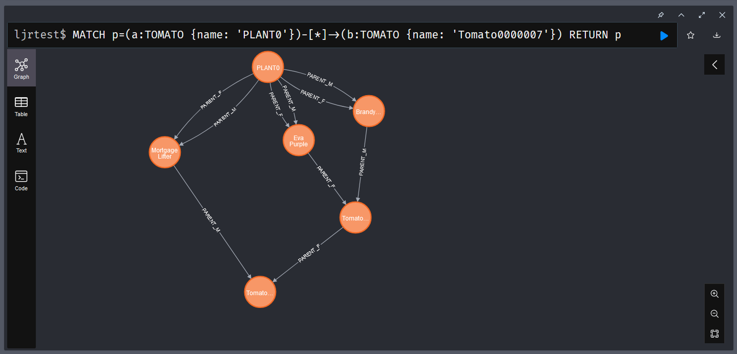
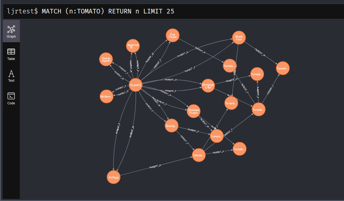
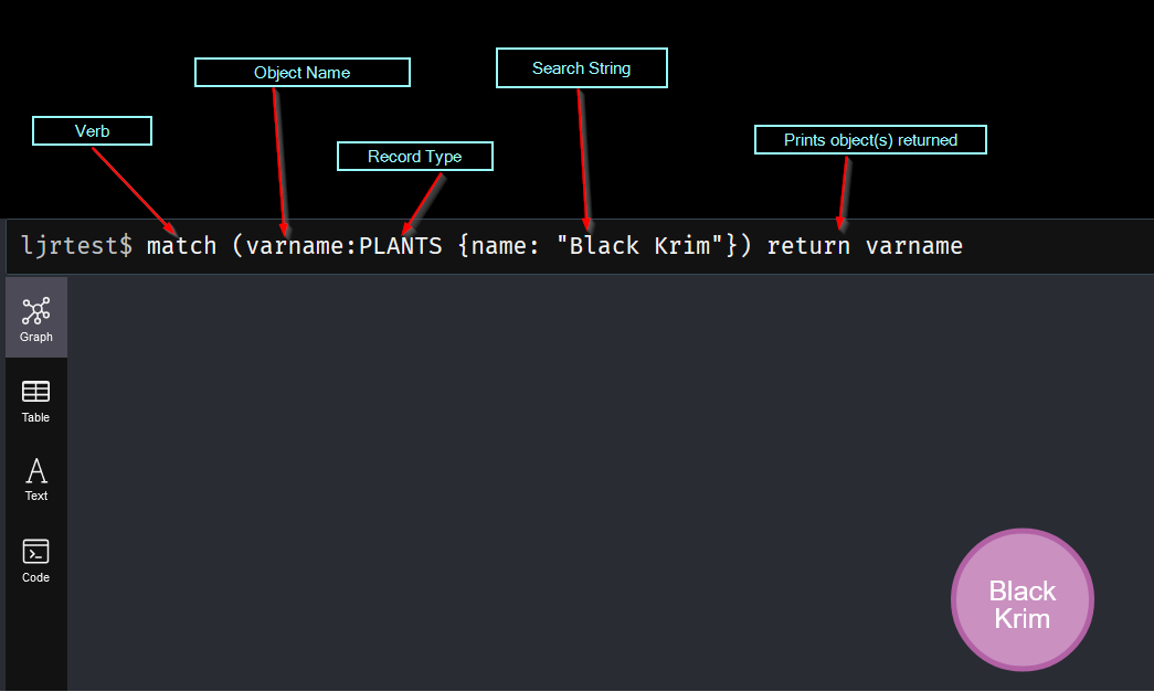
Show records with MATCH

The search starts with the verb “MATCH”. In parenthesis, we add the matching rule. This begins with an object name variable – you can have anonymous nodes (no variable names assigned) by omitting this string and just typing the colon. This is followed by the label that we want to match – basically the type of node we are looking for. Then, in curly braces, a filter – in this case, I am looking for nodes where the “name” field has the value “Black Krim”. Finally, there’s a return statement that indicates that we want to output the matched results.

You can include relationships in the query – parenthesis around nodes and square brackets around relationships.

(placeholdername:nodes)-[:RELATIONSHIP_CONNECTION_TYPE]->(anotherplaceholdername:otherNodes)

This is what makes graph databases interesting for tracking hybridization – we can easily produce the lineage of the plants we develop.

Deleting a record

Deleting a record is used in conjunction with match — use the DELETE verb on the collections of objects returned into your variable name. Here, the variable is ‘x’:

MATCH (x:PLANTS{name: 'Black Krim'})
DELETE x

Deleting a record and relationships by ID

When deleting a record, you can include relationship matches:

MATCH (p:PLANTS) where ID(p)=1
OPTIONAL MATCH (p)-[r]-()
DELETE r,p

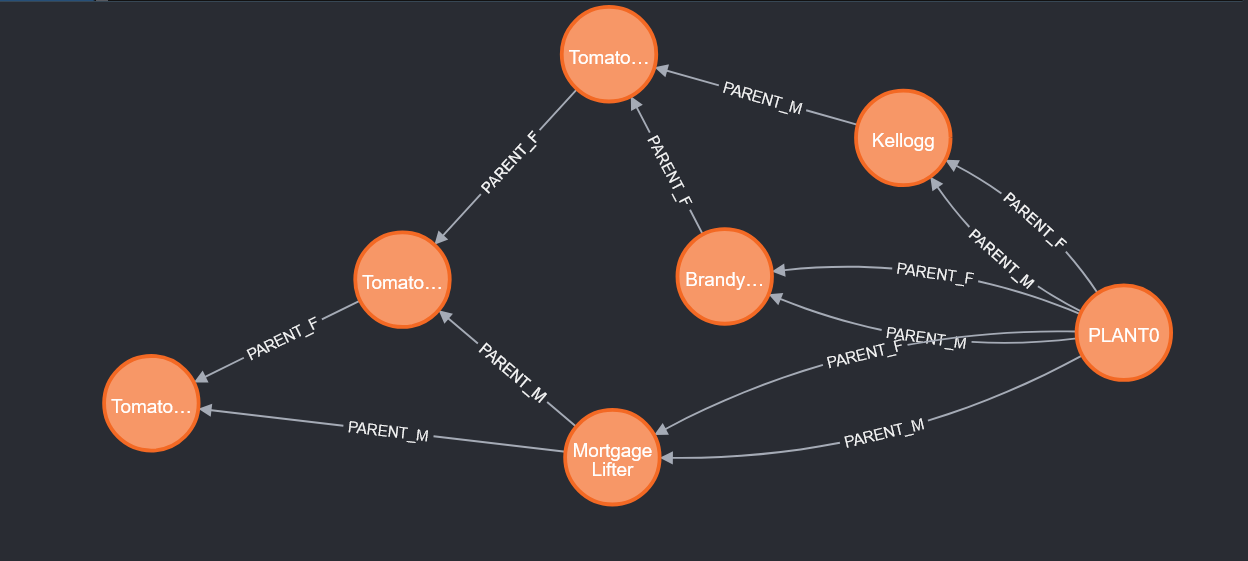
Create a relationship

To create a relationship, we first need to match two objects – here I am finding a plant named PLANT0 and all of the “heirloom seedstock” plants to which I assigned year 1900 – and create parent/child relationships. Since there is both a male and female parent, that is included in the relationship name:

MATCH (a:TOMATO), (b:TOMATO)
WHERE a.name = 'PLANT0' AND b.year = '1900'
CREATE (a)-[r:PARENT_M]->(b)

MATCH (a:TOMATO), (b:TOMATO)
WHERE a.name = 'PLANT0' AND b.year = '1900'
CREATE (a)-[r:PARENT_F]->(b)

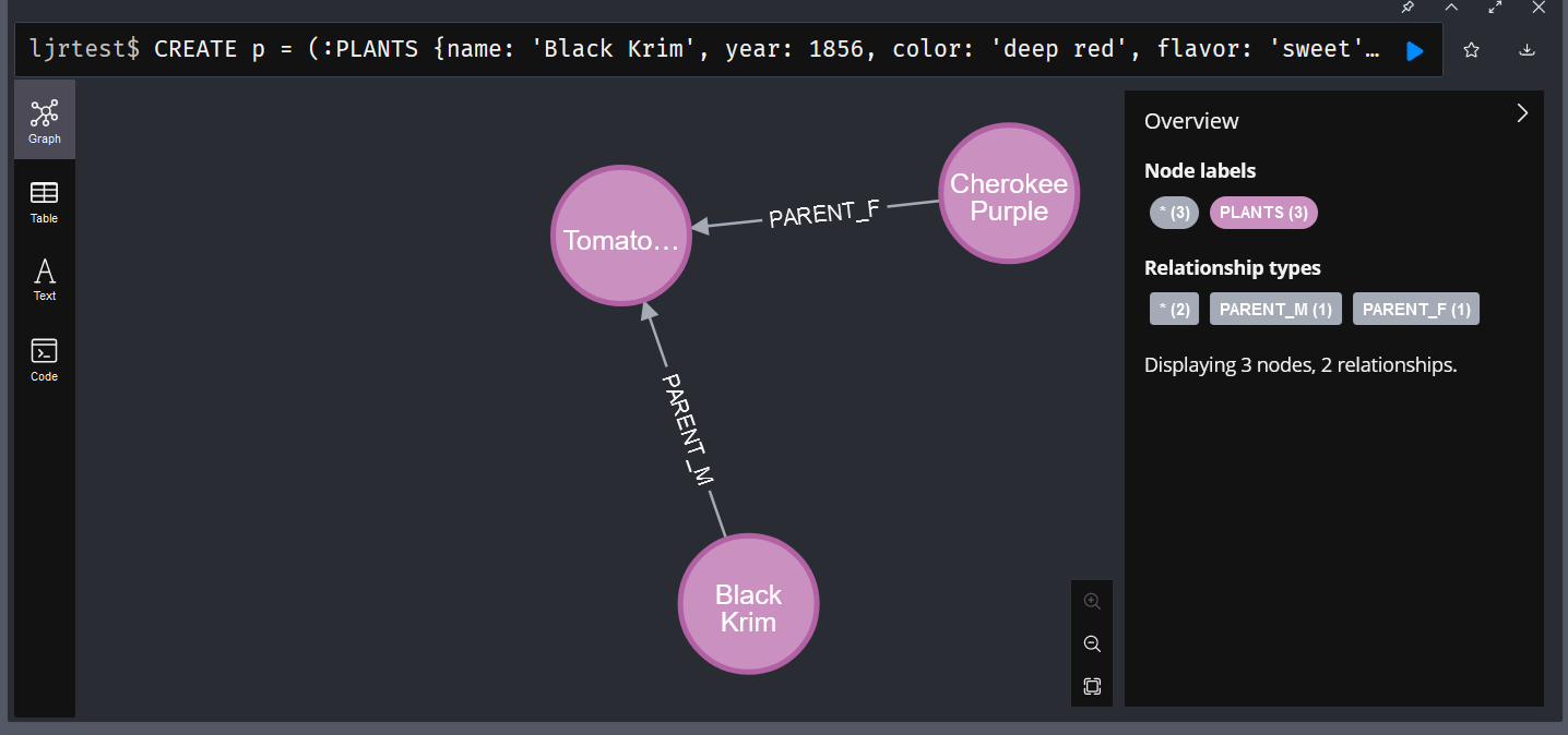
Create records with parent/child relationships

You can create records and relationships in a single command, too:

CREATE p = (:PLANTS {name: 'Black Krim', year: 1856, color: 'deep red', flavor: 'sweet', notes: 'Heirloom seedstock'})-[:PARENT_M]->(:PLANTS {name: 'Tomato0000001', color: 'deep red', flavor: 'sweet', year: '2023', notes: ''})<-[:PARENT_F]-(:PLANTS {name: 'Cherokee Purple', color: 'purple', flavor: 'acidic', year: 1890, notes: 'Heirloom seedstock'})

RETURN p

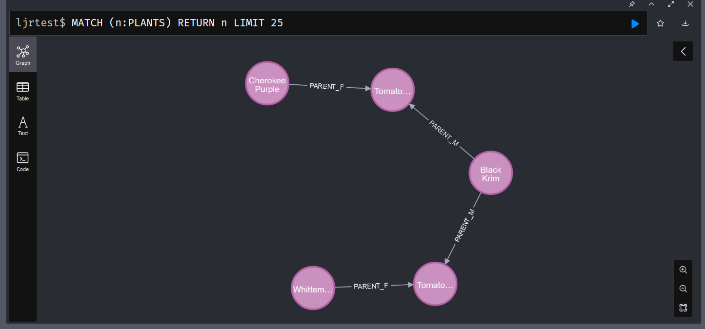
Viewing Records with Relationships

When you match records, you will also get their relationships:

Bulk importing data

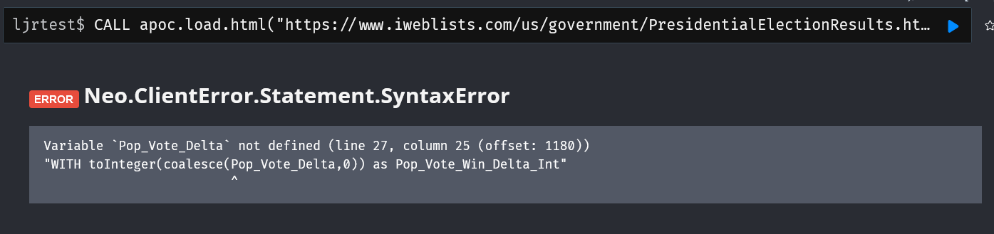
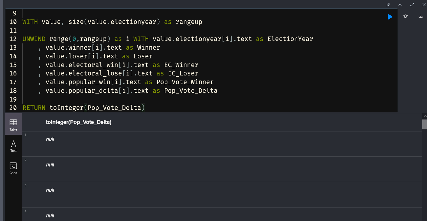
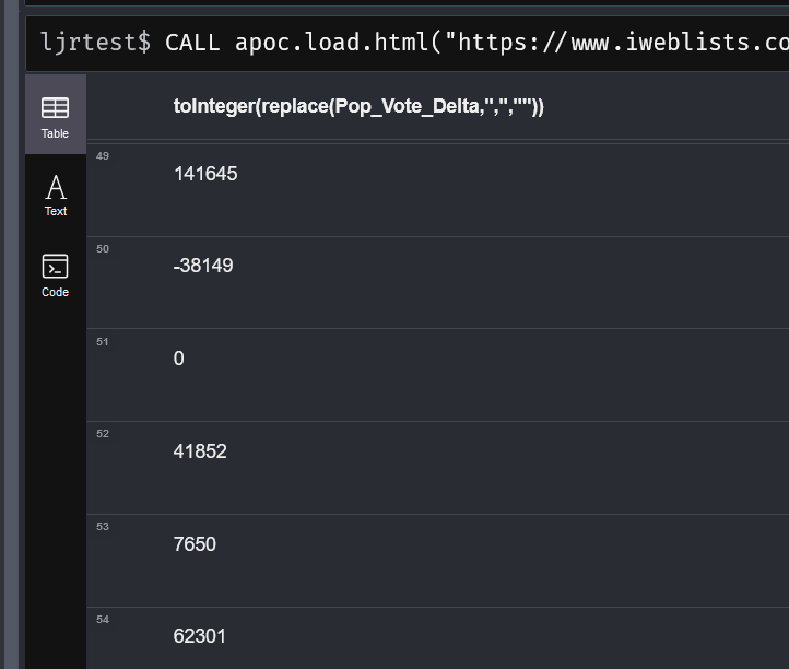
LOAD CSV WITH HEADERS FROM ‘https://www.rushworth.us/lisa/ljr_plant_history.csv’


NEO4J: Basics

When I first encountered the idea of labeled property graph data storage, I thought about the Dirk Gently Holistic Detective Agency series — where a belief in the fundamental interconnectedness of things plays a central role to the plot. Traditional SQL storage stored information and relationships were defined by cross-referencing a field (or more) between tables. The creators of graph databases sought to store the relationships along with data elements.

A labeled property graph database store nodes – the circles below – and define relationships – the lines – between nodes. Relationships are a way to show the interconnectedness of all things — people who purchased items, individuals who acted or directed films. I am looking at graph databases to maintain plant hybridization records — relationships build the family tree.

Nodes can have a label – essentially a classification, here I have “Candidate” nodes and “Election” nodes. A node can have multiple labels — maybe a political party affiliation as well as candidate. Nodes can include relationships to themselves (I’ve met me?)

Relationships have a type – WON or LOST here. Relationships are also directional – an election didn’t win a dude, a dude won an election.

Both nodes and relationships can have properties – additional information about the entity. In this example, each election node stores a year in which the election took place along with the vote totals both popular vote and electoral college results.


Postgresql SPLIT_PART and TRANSLATE

We have a database where there’s a single field, args, into which the vendor has glommed quite a few different things. Unfortunately, I need one of those numbers.

"---
- Workbook
- 4477
- Sample Report
- 18116
- null
"

You can use split_part to break a column into elements and only use one of those elements split_part(column_to_split, delimiter, ColumnToKeep)

As an example:
SPLIT_PART(b.args, E'\n', 3)AS task_workbook_id

In this case, I subsequently needed to eliminate the dash and space that prefixed the line. Using TRANSLATE, I am removing the ‘- ‘ with ”:
TRANSLATE ( SPLIT_PART(b.args, E'\n', 3), '- ','') AS task_workbook_id

And now I’ve just got 4477

Using PG_CRON In PostgreSQL

The pg_cron extension allows you to schedule tasks from within your database (or, to those who didn’t know it was a thing, it allows you to hide {really well} jobs that mutate or remove data leading to absolutely inexplicable database content). While the project documents how to create or remove a scheduled job, I had quite the time figuring out how to see what was scheduled.

To see jobs scheduled in pg_cron:

To see the result of scheduled jobs:

PostgreSQL Wraparound

We had a Postgres server go into read-only mode — which provided a stressful opportunity to learn more nuances of Postgres internals. It appears this “read only mode” something Postgres does to save it from itself. Transaction IDs are assigned to each row in the database — the ID values are used to determine what transactions can see. For each transaction, Postgres increments the last transaction ID and assigns the incremented value to the current transaction. When a row is written, the transaction ID is stored in the row and used to determine whether a row is visible to a transaction.

Inserting a row will assign the last transaction ID to the xmin column. A transaction can see all rows where xmin is less than its transaction ID. Updating a row actually creates a new row — the old row then has an xmax value and the new row has the same number as its xmin — transactions with IDs newer than the xmax value will not see the row. Similarly, deleting a row updates the row’s xmax value — older transactions will still be able to see the row, but newer ones will not.

You can even view the xmax and xmin values by specifically asking for them in a select statement: select *, xmin, xmax from TableName;

The transaction ID is stored in a 32-bit number — making the possible values 0 through 4,294,967,295. Which can become a problem for a heavily I/O or long-running database (i.e. even if I only get a couple of records an hour, that adds up over years of service) because … what happens when we get to 4,294,967,295 and need to write another record? To combat this,  Postgres does something that reminds me of the “doomsday” Mayan calendar — this number range isn’t aligned on a straight line where one eventually runs into a wall. The numbers are arranged in a circle, so there’s always a new cycle and numbers are issued all over again. In the Postgres source, the wrap limit is “where the world ends”! But, like the Mayan calendar … this isn’t actually the end as much as it’s a new beginning.

How do you know if transaction 5 is ‘old’ or ‘new’ if the number can be reissued? The database considers half of the IDs in the real past and half for future use. When transaction ID four billion is issued, ID number 5 is considered part of the “future”; but when the current transaction ID is one billion, ID number 5 is considered part of the “past”. Which could be problematic if one of the first records in the database has never been updated but is still perfectly legitimate. Reserving in-use transaction IDs would make the re-issuing of transaction IDs more resource intensive (not just assign ++xid to this transaction, but xid++;is xid assigned {if so, xid++ and check again until the answer is no}; assign xid to this transaction). Instead of implementing more complex logic, rows can be “frozen” — this is a special flag that basically says “I am a row from the past and ignore my transaction ID number”. In versions 9.4 and later, both committed and aborted hint bits are set to freeze a row — in earlier versions, used a special FrozenTransactionId index.

There is a minimum age for freezing a row — it generally doesn’t make sense to mark a row that’s existed for eight seconds as frozen. This is configured in the database as the vacuum_freeze_min_age. But it’s also not good to let rows sit around without being frozen for too long — the database could wrap around to the point where the transaction ID is reissued and the row would be lost (well, it’s still there but no one can see it). Since vacuuming doesn’t look through every page of the database on every cycle, there is a vacuum_freeze_table_age which defines the age of a transaction where vacuum will look through an entire table to freeze rows instead of relying on the visibility map. This combination, hopefully, balances the I/O of freezing rows with full scans that effectively freeze rows.

What I believe led to our outage — most of our data is time-series data. It is written, never modified, and eventually deleted. Auto-vacuum will skip tables that don’t need vacuuming. In our case, that’s most of the tables. The autovacuum_freeze_max_age parameter sets an ‘age’ at which vacuuming is forced. If these special vacuum processes don’t complete fully … you eventually get into a state where the server stops accepting writes in order to avoid potential data loss.

So monitoring for transaction IDs approaching the wraparound and emergency vacuum values is important. I set up a task that alerts us when we approach wraparound (fortunately, we’ve not gotten there again) as well as when we approach the emergency auto-vacuum threshold — a state which we reach a few times a week.

Using the following query, we monitor how close each of our databases is to both the auto-vacuum threshold and the ‘end of the world’ wrap-around point.

WITH max_age AS ( SELECT 2000000000 as max_old_xid
                        , setting AS autovacuum_freeze_max_age FROM pg_catalog.pg_settings 
                        WHERE name = 'autovacuum_freeze_max_age' )
         , per_database_stats AS ( SELECT datname , m.max_old_xid::int 
                        , m.autovacuum_freeze_max_age::int 
                        , age(d.datfrozenxid) AS oldest_current_xid 
                        FROM pg_catalog.pg_database d 
                        JOIN max_age m ON (true) WHERE d.datallowconn ) 

SELECT max(oldest_current_xid) AS oldest_current_xid 
      , max(ROUND(100*(oldest_current_xid/max_old_xid::float))) AS percent_towards_wraparound 
      , max(ROUND(100*(oldest_current_xid/autovacuum_freeze_max_age::float))) AS percent_towards_emergency_autovac FROM per_database_stats

If we are approaching either point, e-mail alerts are sent.

When a database approaches the emergency auto-vacuum threshold, we freeze data manually —  vacuumdb --all --freeze --jobs=1 --echo --verbose --analyze (or –jobs=3 if I want the process to hurry up and get done).

Postgresql – Querying Hot Standby Server

We hit our maximum connection limit on some PostgreSQL servers — which made me wonder why the hot standby servers weren’t being used … well, at all. They’re equally big, expensive servers with loads of disk space. But they’re just sitting there “in case”.

So we directed some traffic over to the standby server. I’m also going to tweak a few settings related to user limits — increase the max connections since these are dedicated hosts and have plenty of available I/O, memory, CPU, etc resources; increase the number of reserved connections since replication filled up all of the reserved slots; implement a per-user connection limit on one account that runs a lot of threads — but directing some people who were only trying to look at data over to the standby server seemed like a quick fix.

Now, we discovered something interesting about how queries against the standby interact with replication. It makes a lot of sense when you start thinking about it — if you query against the writable replica, there’s some blocking that goes on. The system isn’t going to vacuum data that you’re currently trying to use. The standby, however, doesn’t have any way to clue the writable replica in to the fact you are trying to use some data. So the writable replica gets a delete, does its thing to hide those rows from future queries, and eventually auto-vacuum comes through and cleans up those rows. All of this gets pushed over to the standby … and there goes the data you were trying to read.

Odds of this happening on a query that takes eight seconds? Incredibly low! Odds increase, however, the longer a query runs. So some of our super massive reports started seeing an error indicating that their query was cancelled “due to a conflict with recovery”

There are two solutions in the PostgreSQL documentation — one is to increase the max_standby_streaming_delay value (there’s also an archive delay, but we aren’t particularly concerned about clients querying the server during recovery operations) the other is to avoid vacuuming data too quickly — either by setting hot_standby_feedback on the standby or increasing vacuum_defer_cleanup_age on the primary.

There’s a third option too — don’t use the standby for long-running queries. That’s easily done in our case … and doesn’t require tweaking any PostgreSQL settings. Ad hoc reporting and direct user access really shouldn’t be implementing such substantial queries (it’s always good to have a SQL expert plan out and optimize complex queries if that’s an option).

Analyzing Postgresql Tmp Files

Postgresql stores temporary files for in-flight queries — these don’t normally hang around for long, but sorting a large amount of data or building a large hash can create a lot of temp files. A dead query that was sorting a large amount of data or …. well, we’ve gotten terabytes of temp files associated with multiple backend process IDs. The file names are algorithmic — a string “pgsql_tmp followed by the backend PID, a period, and then some other number. Thus, I can extract the PID from each file name and provide a summary of the processes associated with temp files.

To view a summary of the temp files within the pgsql_tmp folder, run the following command to print a count then a PID number:
ls /path/to/pgdata/base/pgsql_tmp | sed -nr 's/pgsql_tmp([0-9]*)\.[0-9]*/\1/p' | sort | uniq -c

A slightly longer command can be used to reverse the columns – producing a list of process IDs followed by the count of files for that PID – too:
ls /path/to/pgdata/base/pgsql_tmp | sed -nr 's/pgsql_tmp([0-9]*)\.[0-9]*/\1/p' | sort | uniq -c | sort -k2nr | awk '{printf("%s\t%s\n",$2,$1)}END{print}'