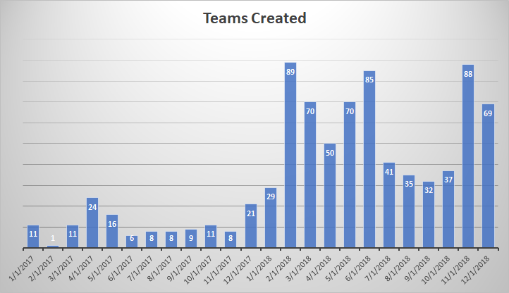
Did you know … you can use Microsoft Excel to count the number of records within a range?

I’ve been generating reports to track our Microsoft Teams adoption – how many people are using Teams, how many messages are being sent in Teams, how many Teams are there. Some of these metrics have easily visualized count-per-unit-time summaries available. Some, like the number of Teams, do not.

Team	Created On
Directory Services	1/19/2017
App Proxy	1/19/2017
LDAP	1/19/2017
ADFS	1/19/2017
Nagios	1/19/2017
File Cluster	1/19/2017
Exchange Online	1/19/2017
Active Directory	1/19/2017
Commvault	1/19/2017

But it’s easy to turn a list of groups and creation dates into visualizable data. Paste the data into Excel. To find the number of items where “Created On” falls in a range, we need to be able to define that range. 01 January 2017 is easy enough, but how do you get the end of January? Excel has a function, EOMONTH, that returns the last day of a month.

Date is any date object. Offset is an integer number of months prior (negative numbers) or after (positive numbers) Date for which you want the last day of the month. I can list the dates to start and end quarters with =EOMonth(Date,2). With 01 January 2017 in cell D2, the last day of January is =EOMonth(D2,0)

I don’t want to type01 Feb, Mar, April … flash fill and the fill handle need a few values before they can figure out the rest of a sequence. But I can use the last day of the month to get the first day of the next month – just add one! With 31 January 2017 in cell E2, I want =E2 + 1 in cell D3. (Yes, there are other ways to do this – probably dozens.)

Now that we’ve got a formula for the start and end of the month, just fill down to produce the ranges we need to see how many Teams were created each month. Then we just need a formula to do the counting for us. I use the COUNTIFS function.

=COUNTIFS($B$2:$B$1000,”>=”&D2,$B$2:$B$1000,”<=”&E2)

Counts the number of items in the range $B$2:$B$1000 (the cell range is static as the formula is copied elsewhere, hence the